Tag: CFD setup mistake

Turbulence Model Selection in CFD: A Practical Guide to Choosing the Right Model

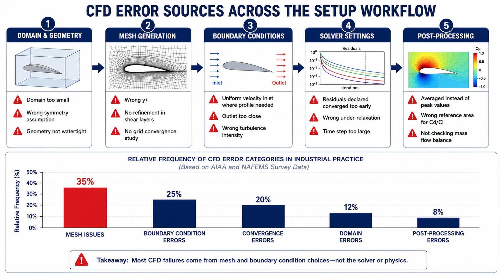
Two engineers open the same CFD solver for the first time. One picks k-omega SST because that’s what the tutorial used. The other picks LES because it sounds more accurate. Three days later, the first engineer has a converged result within 5 percent of the experimental reference. The second engineer’s simulation is still running, has burned through 40 times more compute time, and is showing instabilities because the mesh was never designed for LES.

Neither engineer understood what actually drives the choice.

Quick answer: There is no single best turbulence model. The right choice depends on whether your flow is attached, mildly separated, or massively separated. Attached flow (aircraft cruise, pipe flow) works well with k-omega SST or Spalart-Allmaras. Massively separated flow (bluff bodies, post-stall wings, aeroacoustics) needs DES or LES, since RANS models cannot represent large-scale unsteady separation correctly at any mesh resolution.

Turbulence model selection is one of the most consequential decisions in CFD setup, and one of the least understood outside fluid dynamics specialists. The names are intimidating, the math involves closure assumptions most mechanical engineers never studied in depth, and solver documentation tends to be dense and hedged. This guide gives you a practical framework instead: what each model does, when it works, and how to choose for your specific problem.

Why Turbulence Needs Modelling

Turbulent flow is chaotic. At any point, velocity fluctuates rapidly around a mean value, across a huge range of scales at once. Large eddies, the size of the flow geometry, break down into medium eddies, then small eddies, all the way to the Kolmogorov scale, where turbulent kinetic energy finally dissipates into heat.

In a turbine passage, large eddies might span a centimetre. The Kolmogorov scale might be 10 to 50 micrometres. That’s roughly a 1,000-to-1 ratio in length, which becomes a 10⁹ ratio in required computational cells across three dimensions.

This is why turbulence gets modelled instead of resolved directly. The Navier-Stokes equations describe turbulence exactly, but solving them exactly, called Direct Numerical Simulation (DNS), requires meshes of 10¹² to 10¹⁶ cells and thousands of years of compute time at engineering Reynolds numbers. DNS is reserved for low-Re academic research and model calibration. Every practical engineering simulation needs a modelling strategy.

Three Strategies for Handling the Eddy Cascade

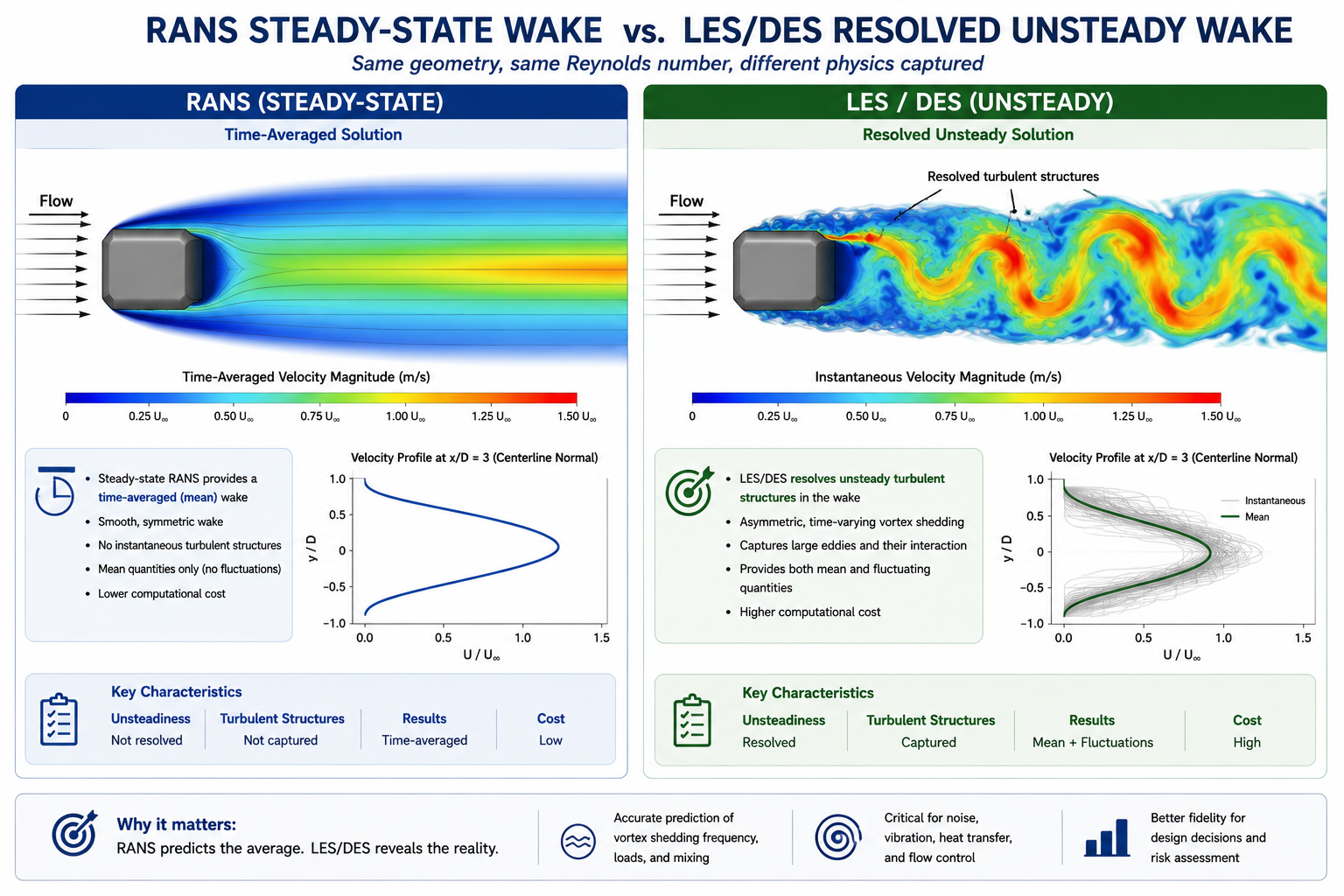
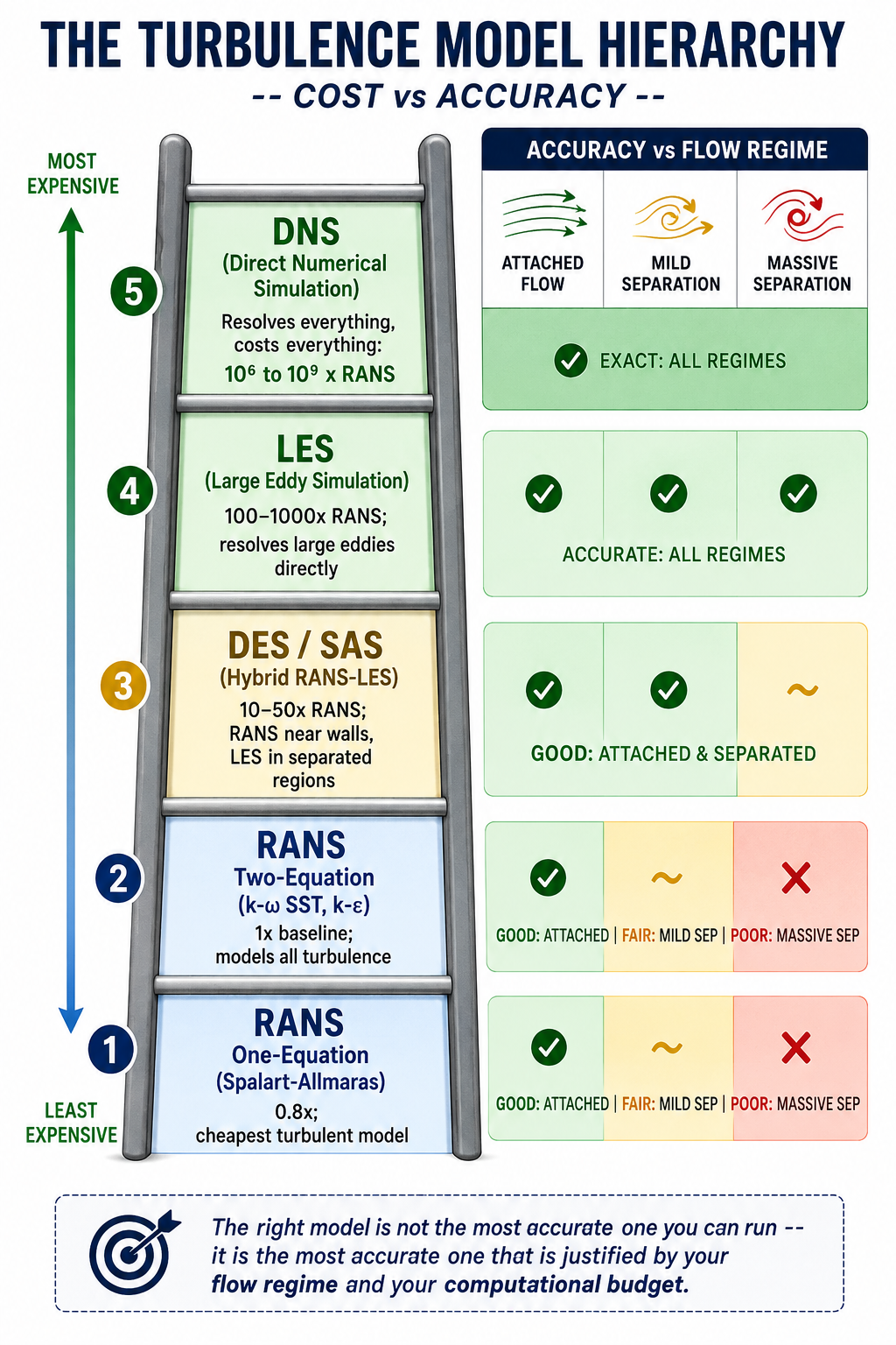
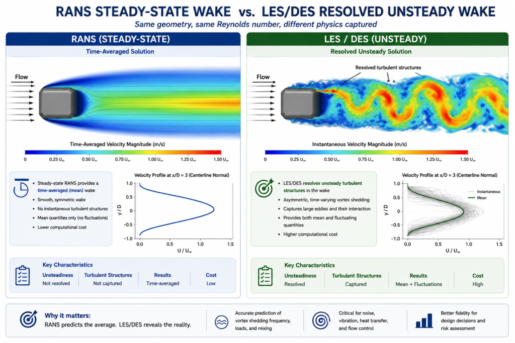
Model everything (RANS). Reynolds-Averaged Navier-Stokes models time-average the governing equations, removing turbulent fluctuations and replacing their effect with a turbulent viscosity term. RANS gives a single steady-state flow field. It’s the fastest approach and handles attached or mildly separated flow well.

Resolve the large eddies, model the small ones (LES and hybrids). Large Eddy Simulation filters the equations to resolve large, energy-containing eddies directly while modelling only the sub-grid scale eddies. It’s far more accurate than RANS for separated flows, but cost scales roughly with Re², making full LES impractical for high-Reynolds-number engineering problems.

Hybrid RANS-LES. Methods like Detached Eddy Simulation (DES) and Scale-Adaptive Simulation (SAS) use RANS near walls, where it’s accurate and cheap, and switch to LES-like behavior in separated regions, where large unsteady eddies dominate. This captures the physics that matters most at roughly 10 to 50 times RANS cost, versus 100 to 1,000 times for full LES.

RANS Models: The Workhorses of Industrial CFD

RANS handles the large majority of engineering CFD work, from automotive aerodynamics to HVAC design to turbomachinery. Knowing what each model is calibrated for, and where it breaks down, is the core practical knowledge.

Spalart-Allmaras: One Equation, One Purpose

Developed by Spalart and Allmaras at Boeing in 1992, this is the simplest widely used turbulence model. It solves a single transport equation for turbulent kinematic viscosity directly, skipping the k-epsilon or k-omega equations. That makes it the cheapest and most numerically robust RANS option.

SA was built specifically for external aircraft aerodynamics in attached or mildly separated flow, calibrated on flat plate and aerofoil boundary layers. It remains standard in NASA’s CFD codes. It is not designed for free shear flows, strongly separated flows, or anisotropic turbulence. Using it on a bluff body or a post-stall wing will produce wrong results no matter how good the mesh is.

The k-epsilon Family: Robust but Flawed Near Walls

Standard k-epsilon (Jones and Launder, 1972) was the first widely adopted two-equation model and remains common in non-aerospace industrial CFD. Its known weakness is poor near-wall behavior: the epsilon equation goes singular near the wall, forcing reliance on wall functions and limiting its usefulness where near-wall physics matters. In adverse pressure gradients, it over-predicts skin friction and delays predicted separation.

Realizable k-epsilon (Shih et al., 1994) improves on this by making the C_mu coefficient vary with local strain rate and enforcing mathematical realizability constraints. It performs noticeably better for round jets, mixing layers, and mildly separated flows, making it the preferred choice for combustion chambers and industrial internal flows.

k-omega SST: Why It Became the Default

Developed by Florian Menter and published in 1994, k-omega SST is now the standard model for industrial external aerodynamics and the default in most general-purpose solvers. It fixes the two biggest weaknesses of its predecessors: k-epsilon’s poor near-wall behavior and standard k-omega’s oversensitivity to freestream conditions.

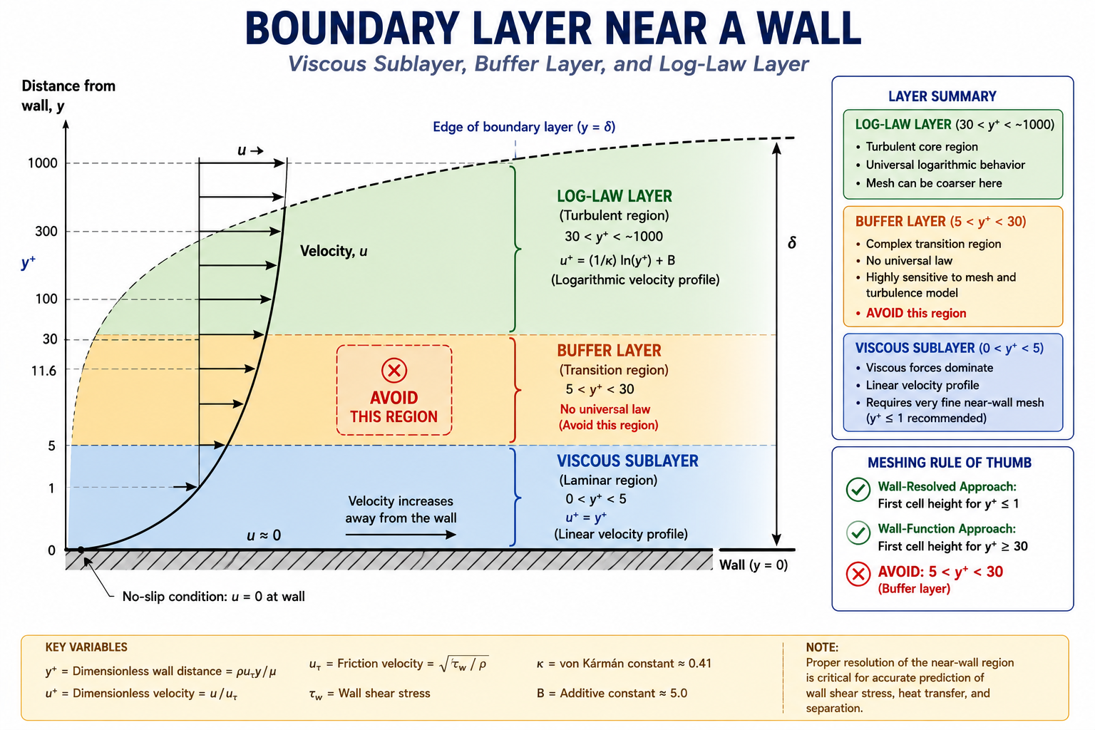
SST does this with a blending function that transitions between k-omega near walls, where it gives excellent near-wall accuracy without wall functions at y+ below 1, and k-epsilon in the freestream, where it’s more robust. The switch is automatic based on wall distance. A built-in stress limiter also prevents over-production of turbulent viscosity in adverse pressure gradients, one reason SST predicts separation onset more accurately than either parent model, as detailed in Menter’s original AIAA paper introducing the model.

SST isn’t perfect. It still under-predicts separation onset in strongly adverse pressure gradients and misrepresents massively separated flow. A cylinder in crossflow, a stalled wing, or a blunt truck rear will all produce results that mesh refinement cannot fix. Those cases need a higher-fidelity model, or explicit acknowledgment that the RANS result carries large uncertainty.

Reynolds Stress Model: When Anisotropy Matters

Two-equation models rely on the Boussinesq assumption, that turbulent stress is proportional to mean strain rate. That assumption breaks down under strong swirl, curvature, buoyancy, or multiple concurrent shear stresses.

The Reynolds Stress Model solves transport equations for all six Reynolds stress components directly, abandoning Boussinesq. It handles anisotropic turbulence correctly, which helps for rotating machinery, strongly swirling combustors, and buoyancy-driven flows. The cost is 3 to 5 times higher than two-equation models, and it’s numerically less stable. For most industrial work, the accuracy gain over SST doesn’t justify the cost. Reserve RSM for cases where anisotropy is the governing physics, not a minor correction.

The 10-Model Comparison

Cost is relative to standard k-epsilon at equivalent mesh density. Accuracy is assessed separately for attached and separated flow, since these are fundamentally different challenges for a turbulence model.

Model	Type	Cost vs RANS k-e	Attached Flow Accuracy	Separated Flow Accuracy	Best Use Case	Avoid When
Spalart-Allmaras	RANS	0.8x	Good for thin boundary layers	Poor	Thin airfoil, attached aero	Any significant separation
k-epsilon (standard)	RANS	1.0x	Moderate; poor near walls	Poor	Internal duct/pipe flows	Near-wall or adverse gradient regions
k-epsilon (Realizable)	RANS	1.05x	Better for jets	Still poor for massive separation	Jet mixing, combustion	High-AoA aerodynamics
k-omega (standard)	RANS	1.0x	Excellent near-wall	Poor in freestream	Near-wall/transitional flow	Freestream-dominated problems
k-omega SST	RANS	1.1x	Excellent	Moderate	Default for most external/internal flow	Massively separated/bluff wake flows
Reynolds Stress Model	RANS	3-5x	Excellent for anisotropic turbulence	Better than 2-eq	Rotating machinery, swirl, buoyancy	General use (high cost, marginal gain)
DES	Hybrid	10-50x	Good	Good	High AoA, bluff bodies, separated wakes	Thin boundary layers, unrefined RANS zone
SAS	Hybrid	5-20x	Good	Good for massive separation	DES alternative	Weakly separated flows
LES	Scale-resolving	100-1000x	Excellent	Excellent	Aeroacoustics, fundamental studies	High-Re engineering flows (Re > 10^6)
DNS	Exact	10^6-10^9x	Exact	Exact	Academic turbulence research	Any engineering application

When RANS Isn’t Enough: DES, SAS, and LES

If a flow has large-scale, energetic, unsteady separation that governs the quantity you care about (drag, pressure fluctuation, noise, heat transfer in a separated region), RANS gives the wrong answer regardless of which two-equation model you pick. Time-averaging removes exactly the dynamics that dominate these flows.

Detached Eddy Simulation: The Practical Hybrid

Introduced by Spalart and colleagues in 1997, DES uses RANS in the attached boundary layer and switches to LES-like treatment in the separated region, based automatically on local mesh size relative to the model’s length scale. The widely used variant, Delayed DES (DDES), adds a shielding function to stop the model from switching to LES prematurely inside thick boundary layers, which early DES implementations sometimes did, causing modelled stress depletion and incorrect wall shear stress.

DES gives significantly better results than SST for bluff body aerodynamics, aerofoils near stall, and any separated flow where force coefficients or vortex structure matter. The 10 to 50 times cost penalty is real but manageable for problems where RANS produces 20 to 30 percent errors.

LES: When Only Resolved Unsteady Physics Will Do

LES is the right choice for aeroacoustics, where noise comes from turbulent pressure fluctuations at frequencies RANS can’t resolve, and for heat transfer in highly unsteady separated regions. Its biggest constraint is the near-wall mesh requirement: at Re = 10⁶, wall-resolved LES needs cell sizes on the order of micrometres, making a full vehicle or aircraft prohibitively expensive. Wall-modelled LES (WMLES), which blends a RANS-like near-wall model with outer-region LES, reduces this cost and is an active area of commercial solver development.

Scale-Adaptive Simulation: A DES Alternative

SAS, developed by Menter and Egorov, adds a von Karman length scale term to the omega equation instead of relying on DES’s grid-based trigger. It activates when the local flow length scale drops below the RANS equilibrium scale, letting the model resolve turbulent structures without needing a carefully designed RANS-to-LES transition mesh. In practice, SAS gives similar results to DES for strongly separated flows and is often more robust in transition regions.

Turbulence Model Selection for 12 Engineering Applications

This table is a starting reference, not a substitute for project-specific validation.

Engineering Problem	Recommended Model	Why	Watch For
Aircraft wing at cruise	k-omega SST	Best near-wall accuracy for attached flow	May predict separation 2-3° too late at high AoA
Automotive exterior (sedan)	SST for baseline; DES for wake detail	SST gives Cd within 5-8%; DES resolves unsteady wake	SST can under-predict blunt-rear separation by 10-20%
Circular cylinder in crossflow	DES or LES	RANS misrepresents wake width and shedding frequency	Run at least 10 shedding periods before extracting statistics
Internal pipe flow (developed)	k-omega SST or Realizable k-epsilon	Well-captured by either two-equation model	Confirm y+ matches chosen near-wall treatment
HVAC room airflow	SST with Boussinesq buoyancy	Standard for room CFD; buoyancy term essential	Diffuser modelling detail strongly affects jet throw
Wind around a tall building	SST with ABL modifications; LES for pedestrian comfort	Handles time-averaged wind loads	Inlet profile must match ABL log-law and roughness
Gas turbine blade cooling	SST with gamma-Re_theta transition	Captures laminar-to-turbulent onset for heat transfer	Requires accurate inlet turbulence intensity
Centrifugal pump impeller	SST in rotating frame (MRF or sliding mesh)	Handles body forces and secondary flows	Needs rotation-corrected turbulence production term
Combustion chamber / burner	Realizable k-epsilon or RSM with combustion model	Compatible with combustion models; RSM better for swirl	Include radiation model for high-temperature flames
Aeroacoustic noise from aerofoil	LES with Ffowcs Williams-Hawkings analogy	Only LES resolves noise-generating structures	Mesh must resolve eddies at frequencies of interest
Ship hull resistance	SST with Volume of Fluid (VOF)	Standard for hydrodynamics; VOF captures wave resistance	Free surface mesh needs 20+ cells per wave height
Blood flow through a stent	Laminar/transitional SST with Carreau non-Newtonian model	Physiological Re is mostly laminar to transitional	Requires pulsatile BCs from measured waveforms

Understanding Model Constants

Every turbulence model contains empirical constants calibrated against experimental data for specific canonical flows. These aren’t free parameters to tune for a better match on one result. Adjusting them to fit a specific experiment is curve-fitting, not physics, and the modified constants will produce wrong results for any flow outside the case they were tuned to.

Model	Key Constant	Default	Controls	When to Modify
k-omega SST	a1 (stress limiter)	0.31	Max ratio of shear stress to k	Rarely; some codes use 0.302
k-omega SST	beta* (k dissipation)	0.09	Dissipation-to-k-omega relationship	Never
k-epsilon standard	C_mu	0.09	Overall turbulence level	Sometimes 0.06-0.07 for round jets
k-epsilon standard	C1_epsilon, C2_epsilon	1.44, 1.92	Production/destruction in epsilon equation	Only with specific swirl validation
Spalart-Allmaras	cb1, cb2, cv1	0.1355, 0.622, 7.1	Production, destruction, viscosity ratio	Only for transition modeling

The only legitimate reasons to change a constant: a published, peer-reviewed modification exists for a known model deficiency in your specific flow class, or you’re calibrating a transition model against measured data for one specific geometry and condition. Any other adjustment turns the simulation into result-tuning with zero predictive value for new conditions, even if it matches the calibration case perfectly.

Laminar-to-Turbulent Transition

Standard RANS models assume fully turbulent flow from the inlet. That’s fine at high Reynolds numbers, but for gas turbine blades at altitude, fan and compressor blades, low-speed wind turbine aerofoils, and small propellers, a meaningful part of the surface may still be laminar. Treating it as turbulent overestimates skin friction and misrepresents heat transfer.

The gamma-Re_theta transition model, developed by Menter, Langtry, and colleagues as an add-on to SST, solves two extra transport equations: one for intermittency (the fraction of time flow is turbulent at a point) and one for the transition momentum thickness Reynolds number. It compares local flow conditions against empirical transition-onset correlations and progressively activates the full turbulence model across the transition region.

This model matters most for gas turbine blade heat transfer, where laminar-versus-turbulent regions shift the local Nusselt number by a factor of 3 to 5, and for low-speed aerofoil performance, where leading-edge laminar separation bubbles govern maximum lift. It adds roughly 20 percent compute cost and needs correct freestream turbulence intensity to predict bypass transition accurately.

Practical Setup: Getting the Inlet Values Right

For k-omega SST, turbulent kinetic energy k and specific dissipation rate omega must be set at every inlet. Getting them wrong rarely causes divergence, but it shifts turbulence levels throughout the domain, especially near separated regions.

GIVEN: Freestream velocity V, turbulence intensity Tu, length scale L

k = 1.5 * (V * Tu)^2
Example: V=50 m/s, Tu=0.005 -> k = 1.5 * (0.25)^2 = 0.9375 m^2/s^2

omega = k^0.5 / (C_mu^0.25 * L), where C_mu = 0.09
Example: k=0.9375, L=0.01m -> omega ≈ 176.6 s^-1

epsilon = C_mu^0.75 * k^1.5 / L (for k-epsilon)
Example: k=0.9375, L=0.01m -> epsilon ≈ 14.9 m^2/s^3

Turbulent viscosity ratio target: 1-10 for low-Tu freestream; 10-100 for internal flows

Turbulence intensity guide:

Low-turbulence wind tunnel: 0.05 to 0.3 percent
Atmospheric boundary layer: 5 to 15 percent
Industrial pipe/duct flow: 3 to 8 percent
Turbomachinery inlet: 3 to 10 percent
Combustion chamber inlet: 5 to 20 percent

Turbulent length scale guide:

Pipe/duct flow: 0.07 × hydraulic diameter
Flat plate: 0.4 × boundary layer thickness
Wind tunnel: 0.01 × tunnel width
Atmospheric: 100 to 300 m at reference height

Steady RANS vs. URANS

URANS is appropriate when large-scale unsteadiness is periodic and much larger in scale than turbulence itself: vortex shedding, periodic stall, pulsatile pipe flow. It’s not a substitute for LES. It still models all turbulence, but lets large-scale unsteady structure develop instead of being averaged away.

If a steady RANS run oscillates and won’t converge, that’s a signal the flow is unsteady, not a convergence problem to push through with more iterations. Either time-average a URANS result or move to DES or LES. An arbitrary instantaneous snapshot of an unsteady solution has no defined physical meaning.

Running a Turbulence Model Sensitivity Study

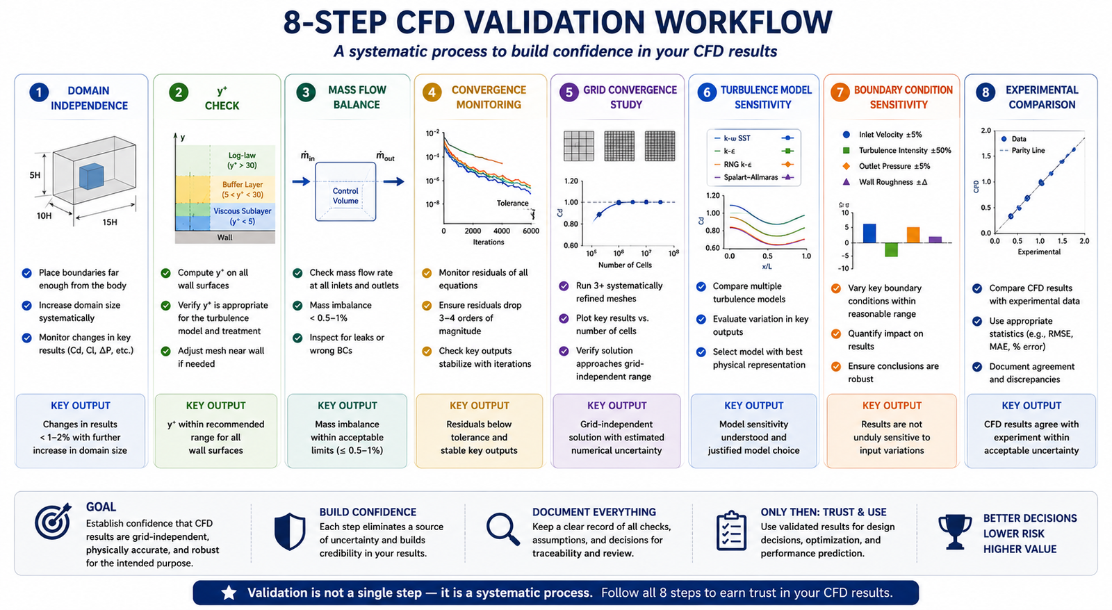
For any result feeding a design decision, run the same geometry, mesh, and boundary conditions through two or three models (say, SST, Realizable k-epsilon, and Spalart-Allmaras for external aero) and compare. Agreement within 5 percent for Cd and 2 percent for Cl means turbulence model choice isn’t the dominant uncertainty. Disagreement above 10 percent means it is, and the choice needs justification against experimental or higher-fidelity data.

A Cp comparison along the surface also shows where the models diverge: leading edge points to transition or stagnation issues, suction surface points to adverse pressure gradient handling, trailing edge points to separation and base pressure.

Worked Examples

Wind load on a low-rise industrial building: A team needed pressure coefficients on a 10m tall, 40m wide, 20m deep building in open terrain for structural loading. They used k-omega SST with an ABL inlet profile matched to a roughness length of 0.03m, generating 15 percent turbulence intensity at roof height. Time-averaged Cp on windward and side walls landed within 10 to 15 percent of wind tunnel data, adequate for code compliance.

The roof was the exception: leading-edge separation over the first 20 to 30 percent of the roof width under-predicted suction by 15 to 25 percent, since SST can’t fully capture that separated zone. LES or wind tunnel data would be needed if the roof were the governing structural case.

Pump impeller at part-load: At 60 percent of design flow, incidence angle at the impeller inlet risked leading-edge separation and rotating stall. The team used SST in a rotating reference frame with sliding mesh for full transient impeller-volute interaction, since steady MRF averages away the tongue-blade interaction that dominates at off-design. Running through 5 impeller revolutions after reaching a stationary state gave head and efficiency predictions within 3 to 5 percent and 2 to 3 percentage points of the test curve at design point, with correct off-design trends even where absolute values differed by 5 to 10 percent.

Frequently Asked Questions

What is the best turbulence model for CFD? There isn’t one. k-omega SST is the industry standard for attached or mildly separated external aerodynamics. Massively separated flows need DES or LES. Aeroacoustics requires LES, since RANS can’t predict the pressure fluctuations that generate noise. Start with SST, validate against a reference, and upgrade only when SST shows a real discrepancy in the regime that matters.

What’s the difference between k-omega and k-omega SST? Standard k-omega has excellent near-wall behavior but is highly sensitive to the omega value set at the freestream inlet, which makes it unreliable for external flows. SST blends k-omega near walls with k-epsilon in the freestream, switching automatically based on wall distance, and adds a stress limiter that improves separation prediction. That combination is why SST outperforms both parent models for external aerodynamics.

When should I use DES instead of RANS? When the flow is separated over a significant area at your operating condition, and the drag, pressure distribution, or acoustic output you’re predicting depends on the structure of that separated region. Common triggers: bluff bodies with large wakes, aerofoils within 3 to 5 degrees of stall, deployed flaps or spoilers, and any case where unsteady loads or vortex structure matter. Budget 10 to 50 times the cost of SST.

Can I use RANS for unsteady problems? Yes, as URANS, when the dominant unsteadiness is large-scale and periodic, like vortex shedding or pulsatile flow. It’s not appropriate when the unsteadiness comes from the turbulence itself or from separated-region dynamics at a scale close to the turbulence scale; those cases need DES or LES.

How much does turbulence model choice affect the final result? For attached flow, different RANS models typically agree within 3 to 8 percent for drag and 1 to 3 percent for lift, so model choice isn’t the dominant error source. For separated flows, RANS models can disagree by 20 to 50 percent, making model choice the largest source of uncertainty. For acoustics, RANS is wrong by orders of magnitude regardless of model, since it averages away the noise source entirely.

What does y+ have to do with turbulence model selection? Different models need the first wall cell in different parts of the boundary layer. Low-Re models and SA need y+ below 1. Standard wall functions need y+ between 30 and 300. Mismatching the mesh to the model, or landing in the 5-to-30 buffer layer, produces wall shear stress errors of 10 to 40 percent regardless of which model you chose. Decide the near-wall treatment before generating the mesh, then check y+ post-solution.

Key Takeaways

Turbulence model selection isn’t about running the most accurate model available. It’s about matching the physics that governs your quantity of interest to a cost justified by the engineering decision at hand. LES on a duct pressure drop wastes compute resolving detail that changes the answer by under 1 percent. SST on a bluff body aeroacoustics problem gives noise predictions wrong by orders of magnitude. Both are the wrong choice, just in opposite directions.

Start by classifying the flow: attached, mildly separated, or massively separated. Attached flow needs SST or SA. Massive separation needs DES or LES. Mild separation needs SST plus a sensitivity study against a higher-fidelity reference. Then check secondary physics: rotation needs correction terms, transition needs the gamma model, strong anisotropy may need RSM. Finally, match the near-wall treatment and mesh to the y+ range that treatment requires.

None of this removes the need for validation against a reference before trusting a result for a design decision. The models here have documented accuracy ranges and known failure modes. Working inside those ranges, with validation, gives reliable results. Working outside them without validation gives results indistinguishable from wrong ones.

August 8, 2026

Common CFD Setup Mistakes and How to Avoid Them (20-Point Guide)

A recent CFD run took four days to set up and 16 hours to run on a 128-core cluster. The predicted drag coefficient was 0.287. The wind tunnel measurement for the same configuration was 0.231. That’s a 24 percent error, and it had nothing to do with turbulence model uncertainty or geometry mismatches.

The real cause was three stacked setup errors: a domain that ended too soon behind the wing, a first-cell y+ value stuck in the unreliable buffer layer, and a convergence call made from residuals alone while the drag coefficient was still drifting. Each error alone would have cost 5 to 10 percent accuracy. Together, they made the result useless for the design decision it was meant to support.

Quick answer: The most common CFD setup mistakes fall into five categories: domain and geometry, mesh quality, boundary conditions, solver settings and convergence, and post-processing. None of them show up as solver errors. The simulation still converges, the plots still look smooth, and the numbers still look plausible. That’s what makes them dangerous, and why systematic checking, not visual inspection, is the only reliable way to catch them.

CFD drag prediction versus wind tunnel measurement showing 24 percent discrepancy caused by CFD setup mistakes errors

CFD setup mistakes happen before the solver ever runs, in decisions about domain size, mesh topology, boundary conditions, and solver parameters. Like FEA preprocessing errors, they produce output that looks completely valid: smooth contours, stable force coefficients, clean convergence histories. The solver never flags them. Only systematic verification, domain independence, mesh independence, y+ checks, mass conservation, and monitored-quantity convergence, can catch them before a bad result reaches a design review.

The 20 Most Common CFD Setup Mistakes at a Glance

The table below lists all 20 mistakes by category, typical error magnitude, how to detect them, and priority. Critical items produce errors above 10 percent and cannot be trusted without correction. High priority items introduce meaningful risk that compounds with other errors. Medium items are good practice that improves reliability and prevents downstream post-processing problems.

#	Mistake	Category	Typical Error	Detection Method	Priority
1	Domain too small	Domain / Geometry	5–30% in force coefficients	Extend boundaries and rerun; compare results	Critical
2	Wrong turbulence model for the regime	Physics	10–50% drag error in separated flow	Compare RANS vs DES/LES against test data	Critical
3	y+ wrong for the near-wall model	Mesh	10–40% skin friction error	Check y+ distribution post-solve	Critical
4	Insufficient mesh in shear layers/wakes	Mesh	10–40% wake drag error	Grid convergence study	Critical
5	Wrong inlet turbulence intensity/length scale	Boundary Conditions	5–20% error in transition/separation	Match Tu and length scale to real conditions	High
6	Outlet too close to the body	Boundary Conditions	Divergence or false backflow	Move outlet 10–20 diameters downstream	Critical
7	Symmetry plane on asymmetric flow	Boundary Conditions	Fundamentally wrong result	Verify symmetry with a full-domain reference run	Critical
8	Wrong pressure-velocity coupling scheme	Solver Settings	Slow convergence or divergence	Use COUPLED for high-Re external aero	High
9	Convergence declared from residuals alone	Convergence	5–25% error	Monitor lift, drag, and mass flow vs. iteration	Critical
10	Too few iterations for steady state	Convergence	Scattered, unstable averages	Run until monitors vary < 0.1% over 200 iterations	High
11	Wrong reference area/velocity for Cd/Cl	Post-processing	Error equal to the ratio of areas used	Document reference values before computing	High
12	Averaged instead of peak values reported	Post-processing	10–40% under-reporting at peaks	Use unaveraged, cell-centred values at critical points	High
13	Wall functions applied at y+ < 30	Mesh	10–30% skin friction over-prediction	Target 30 < y+ < 300 for wall functions	High
14	Missing refinement at leading/trailing edges	Mesh	Wrong pressure distribution, circulation	Cluster mesh at stagnation and wake regions	High
15	Periodic BC on non-periodic flow	Boundary Conditions	Artificial forced periodicity	Verify true periodicity before applying	Medium
16	Wrong fluid properties at operating temperature	Physics	Re error scales all downstream results	Compute Re from actual target conditions	High
17	Time step too large in transient runs	Solver Settings	Aliased or missed unsteady features	Keep Courant number in the recommended range	High
18	Mass flow imbalance not checked	Convergence	Non-physical pressure and force fields	Confirm imbalance < 0.1% of inlet mass flow	Critical
19	Default under-relaxation for all cases	Solver Settings	Divergence or oscillation	Reduce to 0.3–0.5 for difficult problems	Medium
20	No grid convergence study	Mesh	Unknown discretisation error	Run coarse/medium/fine mesh; report GCI	Critical

Category 1: Domain Size and Geometry

Domain size errors are the hardest CFD mistakes to catch from a single run. A domain that’s too small still converges cleanly and looks physically reasonable. The error only surfaces when you enlarge the domain and the results shift, or when you compare against test data and find a systematic bias.

Mistake 1: Domain Too Small

The downstream extent is the dimension analysts underestimate most. If the outlet boundary intersects the wake, or the body’s pressure field reaches it, the outlet condition distorts pressure around the body and skews the drag prediction. Lateral extents should keep blockage ratio below roughly 5 percent.

How to check it: run the original domain, then extend every boundary by 50 percent and rerun. If drag or lift changes by more than 1 percent, the domain was too small. This domain independence study should be standard practice before any result is reported.

Flow Configuration	Inlet Distance	Outlet Distance	Lateral Extent	Top/Bottom Extent
External aerofoil/wing (2D)	10–15 chords	20–30 chords	10–15 chords	10–15 chords
External body (car, building), 3D	5–10 lengths	15–20 lengths	5 widths each side	5 heights + ground clearance
Internal duct/pipe flow	10–20 diameters	30–50 diameters	Wall boundary	Wall boundary
Bluff body (cylinder, facade)	10 diameters	30–40 diameters	10 diameters each side	10 diameters
Turbomachinery blade passage	1–2 chords	2–3 chords	Periodic at blade pitch	Periodic or hub/tip wall
Wind over terrain (ABL)	5–10 building heights	15–20 building heights	5 heights each side	6 heights or to gradient height

Mistake 7: Symmetry Applied to Asymmetric Flow

A symmetry plane halves the computational cost, but only when the physics is genuinely symmetric. Many flows that look symmetric aren’t. A cylinder produces an alternating vortex street. A sphere develops an off-axis wake at moderate Reynolds number. A wing at high angle of attack can separate asymmetrically even with symmetric geometry.

Forcing symmetry on an asymmetric flow produces wrong separation onset, wrong stall angle, and often solver oscillation as it fights the imposed constraint. Test it with a full-domain run and no symmetry plane. If the result is symmetric to within 0.1 percent, the assumption holds.

Category 2: Mesh Quality and Refinement

Mesh errors cause roughly 35 percent of all CFD accuracy problems in industrial practice, making this the single largest error source. Unlike domain errors, mesh errors can be local, affecting only a poorly resolved feature, which makes them harder to catch with a simple sensitivity study.

Mistake 3: Wrong y+ Value for the Near-Wall Treatment

The y+ value of the first wall cell determines which part of the boundary layer that cell sits in. Below 5 is the viscous sublayer. Between 5 and 30 is the buffer layer, where neither wall functions nor low-Re models are accurate. Above 30 is the log-law layer.

Wall functions are only valid in the log-law region, typically y+ between 30 and 300. Landing in the buffer layer produces wall shear stress errors of 10 to 40 percent. Low-Reynolds-number models resolve the sublayer directly but need much finer meshes, usually 15 to 20 cells across the boundary layer with the first cell at y+ below 1.

Near-Wall Treatment	y+ Target	What Happens if Wrong	When to Use
Low-Re (resolves boundary layer)	y+ < 1	1–5: transition error; > 5: wall function takes over	Skin friction drag, heat transfer, turbine cooling
Standard wall functions	30 < y+ < 300	< 30: over-predicts shear; > 300: too coarse	Attached turbulent boundary layers, cruise aero
Enhanced wall treatment	Any, avoid 5–30	Buffer layer wrong for both models	General use when y+ is uncertain
Scalable wall functions	y+ ≥ 11.25 (enforced)	Less accurate than low-Re, but avoids divergence	Coarse meshes, ±10–15% accuracy acceptable

Boundary layer diagram showing y+ zones including the buffer layer to avoid in CFD near-wall meshing

Mistake 20: No Grid Convergence Study

Reporting a single-mesh result as your final answer isn’t defensible engineering practice. Every CFD solution carries discretisation error, the gap between the numerical result on a finite mesh and the true solution on an infinitely fine one. That error can range from 0.1 to 30 percent depending on flow complexity and mesh quality.

The standard method for quantifying it is the Grid Convergence Index (GCI), defined by Celik et al. in the ASME Journal of Fluids Engineering. The procedure: run three systematically refined meshes, compute the observed order of convergence, then calculate GCI as a percentage uncertainty band on the fine-mesh result. Below 3 percent is acceptable for most engineering work. Below 1 percent is the bar for certification-grade results.

Worked example:

Coarse mesh (500,000 cells):   Cd = 0.312
Medium mesh (2,000,000 cells): Cd = 0.295
Fine mesh (8,000,000 cells):   Cd = 0.289

Refinement ratio r = 4^(1/3) = 1.587
Observed order p = ln(|-0.017 / -0.006|) / ln(1.587) ≈ 2.25
Richardson extrapolated Cd ≈ 0.286
GCI (fine mesh) ≈ 1.4%

Result: Cd = 0.289 ± 1.4% (acceptable for engineering; < 3% target)

Category 3: Boundary Condition Errors

CFD boundary conditions prescribe the flow state, velocity, pressure, temperature, turbulence, at every domain boundary. The solver builds the interior solution from those values. Get the boundary wrong, and the interior solution is wrong even if the mesh and turbulence model are perfect.

Inlet BC Type	When Correct	Common Mistake
Velocity inlet (uniform)	Known uniform freestream	Applied to non-uniform duct flow
Velocity inlet (profile)	Complex upstream history matters	Skipped when profile data is available
Pressure inlet	Pressure-driven flow (fans, buoyancy)	Used when mass flow is actually known
Mass flow inlet	Metered or fixed-delivery systems	Used at compressible high-speed inlets
Periodic/cyclic	Truly repeating geometry and flow	Applied without verifying periodicity
Turbulence intensity + length scale	Always required	Left at solver default (5%)

Mistake 5: Wrong Inlet Turbulence Intensity

This is one of the most frequently mis-set boundary parameters, largely because analysts leave it at the solver default of 5 percent instead of matching it to the real upstream source.

Low-turbulence wind tunnel: 0.05 to 0.3 percent
Atmospheric boundary layer: 5 to 20 percent, matched to a log-law profile
Industrial fan or blower discharge: 3 to 8 percent
Fully developed pipe flow: roughly 2 to 5 percent

Using the 5 percent default in a low-turbulence wind tunnel case inflates inlet turbulence energy by a factor of 15 to 100, artificially delaying separation and skewing the stall prediction.

Mistake 6: Outlet Boundary Too Close to the Body

A pressure outlet only behaves correctly when the flow there is roughly parallel with small velocity gradients, conditions that exist well downstream of any wake or recirculation. If the outlet sits too close, the prescribed pressure propagates upstream and distorts the flow around the body.

The tell-tale sign: isobars near the outlet curve toward the boundary instead of running parallel to it. If the wake velocity deficit at the outlet exceeds 5 percent of freestream, move the outlet back. For highly separated flows, that can mean 30 to 50 body diameters downstream, further than most analysts initially expect.

Category 4: Solver Settings and Convergence

These are the most deceptive mistakes because they leave no visible trace in the output. A run with wrong under-relaxation, wrong convergence criteria, or too large a time step looks identical to a correctly configured one.

Mistake 9: Declaring Convergence From Residuals Alone

Residuals measure the global imbalance of the governing equations across every cell. Standard guidance says to run until residuals drop 3 to 4 orders of magnitude. That’s necessary, but not sufficient.

A simulation can show residuals down 6 orders of magnitude while drag is still changing by several percent every 100 iterations. This happens because a small, slowly evolving region, a separation bubble or corner vortex, can be invisible to the global residual while still driving the forces you actually care about. Monitor lift, drag, and mass flow directly. Declare convergence when those stabilize, not when residuals hit a target.

Convergence Indicator	Adequate Value	Recommended Action if Not Met
Residual (continuity)	< 1×10⁻⁴ engineering; < 1×10⁻⁶ high-accuracy	Continue iterating; check mesh quality
Residual (momentum)	< 1×10⁻⁴ engineering; < 1×10⁻⁵ aero	Check mesh; reduce time step for transient
Cd stabilisation	< 0.1% change over last 200 iterations	Continue iterating; consider transient RANS
Cl stabilisation	< 0.1% change over last 200 iterations	Time-average or switch to unsteady
Mass flow imbalance	< 0.1% of inlet mass flow	Check for boundary or geometry errors

Mistake 18: Not Checking Mass Flow Imbalance

Mass conservation is the most basic requirement of any incompressible CFD solution. Inlet mass flow should equal outlet mass flow to within 0.1 percent. A larger imbalance means the run hasn’t converged, or there’s a geometry gap or boundary condition mismatch letting mass leak through a wall.

This is the simplest, most reliable check available and should be the first thing you look at, before force, pressure, or temperature results. If mass isn’t conserved, nothing downstream is trustworthy.

Category 5: Post-Processing Errors

These mistakes happen after a correctly run simulation, in how the results get extracted, displayed, or interpreted. They’re the CFD equivalent of FEA post-processing errors.

Mistake 11: Wrong Reference Values for Force Coefficients

Cd = Drag / (0.5 × ρ × V² × A_ref). The reference area A_ref isn’t universal:

Aircraft: wing planform area
Automobiles: frontal projected area
Bluff bodies: frontal projected area (diameter × length, or πd²/4 for a sphere)
Buildings: depends on loading direction

Using the wrong reference area shifts Cd by the ratio between the correct and incorrect areas, which can be 20 to 50 percent for geometries where planform and frontal area diverge significantly. Document the reference area used before publishing any coefficient, and confirm it matches when comparing across codes or against test data.

Mistake 12: Averaged Instead of Peak Values

Contour plots often average nodal values from surrounding elements. At high-gradient locations, stagnation points, suction peaks, separation onset, that averaging can under-report the true peak by 10 to 40 percent. For surface Cp plots, always pull unaveraged, cell-centred values at critical points. The leading-edge suction peak, in particular, determines boundary layer transition and is exactly where averaging does the most damage.

Eight-step CFD validation workflow from domain independence check to experimental comparison

The CFD Validation Workflow

No single check catches every mistake. Domain independence doesn’t catch y+ errors. y+ checks don’t catch convergence errors. The full workflow runs every check in sequence:

Domain independence: extend each boundary 50 percent and compare Cd, Cl, and surface Cp. Repeat until results change less than 1 percent.
y+ check: plot y+ on all walls after the first converged run and confirm it matches your near-wall model.
Mass flow balance: confirm imbalance is under 0.1 percent of inlet mass flow.
Convergence by monitored quantities: track Cd, Cl, mass flow, and pressure versus iteration, not just residuals.
Grid convergence study: run coarse, medium, and fine meshes and report GCI.
Turbulence model sensitivity: compare two models (for example, SST versus Realizable k-ε). Agreement within 5 percent means model choice isn’t the dominant uncertainty.
Boundary condition sensitivity: vary uncertain inlet turbulence by a factor of 3 and check the impact.
Comparison with reference data: validate against a known analytical or experimental case before trusting the target geometry result.

What a Reportable CFD Result Must Include

A CFD result isn’t ready for an engineering decision unless it documents: domain extent and independence study, mesh count and y+ distribution with GCI, turbulence model and justification, boundary conditions with values, convergence history of monitored quantities, mass flow balance, and reference values for any force coefficients. Without this, the result can’t be peer-reviewed, reproduced, or trusted.

Worked Examples

Domain independence failure, ground vehicle aerodynamics: A team ran a 3D RANS simulation at highway speed with an 8-vehicle-length downstream domain and got Cd = 0.298. Extending to 20 lengths dropped Cd to 0.271, a 9.1 percent change. The outlet had been sitting inside the vehicle’s near-wake, pulling base pressure down and inflating drag. Had the original number been used for a compliance check against a 0.28 target, the vehicle would have failed a target it actually met.

False convergence, aerofoil near stall: A NACA 0015 simulation at 15 degrees angle of attack showed residuals down 4 orders of magnitude after 2,000 iterations, reporting Cl = 1.34. Reviewing the Cl history revealed oscillation between 1.28 and 1.41 with a 150-iteration period, meaning it had never actually converged. Switching to unsteady RANS and time-averaging over five shedding periods gave Cl = 1.31 and Cd = 0.094, 8 percent higher than the false-converged steady value.

Frequently Asked Questions

How do I know if my CFD domain is large enough? Run a domain independence study. Extend every boundary by at least 50 percent and compare drag, lift, and surface pressure. If any coefficient shifts more than 1 percent, the domain was too small. For external aerodynamics, the downstream boundary is usually the critical one: 15 to 20 body lengths for streamlined shapes, 30 to 50 for bluff bodies.

What y+ value should I target? Use y+ = 0.5 to 1.0 for low-Reynolds-number models, or 30 to 100 for standard wall functions. Avoid the 5 to 30 buffer layer regardless of which near-wall treatment you’re using.

Why are my residuals converged but my drag coefficient is still changing? Residuals measure global imbalance, not local flow features. A slowly evolving separation bubble or corner vortex can keep drifting the drag coefficient while contributing almost nothing to the global residual. Monitor drag and lift directly and declare convergence only when they stabilize.

What is the Grid Convergence Index and do I need to compute it? GCI quantifies the discretisation error in your result, how far the numerical answer sits from the theoretical infinite-mesh solution. For anything feeding a design decision, regulatory submission, or published comparison, yes, you need it. A three-mesh study costs roughly three times a single run but gives you a defensible uncertainty bound.

How do I handle backflow at my pressure outlet? Move the outlet farther downstream past the recirculation zone; this is the most reliable fix. If that’s not practical, use a backflow prevention option to prescribe flow direction at the boundary, though this only reduces the boundary effect rather than eliminating the underlying accuracy problem.

What turbulence model should I use? k-ω SST is the standard general-purpose choice for external aerodynamics. For strongly separated flows, switch to DES or LES at significantly higher computational cost. Avoid standard k-ε for external aero; it has worse near-wall behavior than SST with no real advantage.

Key Takeaways

CFD setup mistakes happen before the solver runs and produce output that looks completely valid. The 20 mistakes covered here, from an undersized domain through false convergence, account for most CFD accuracy failures in industrial practice. Each has a clear detection method and a known fix.

Build the verification workflow into your process from the first run, not as damage control after someone questions the result. Domain independence and y+ checks cost one or two extra runs. A GCI study costs about three times a single run. Convergence monitoring costs nothing beyond plotting force coefficients alongside residuals. That’s a small price for results with a documented, defensible uncertainty bound.

August 6, 2026