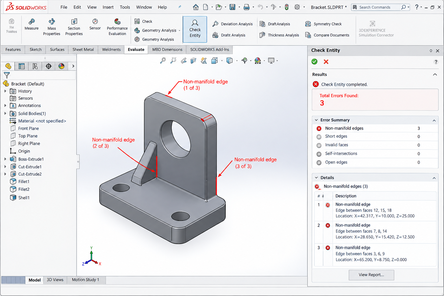
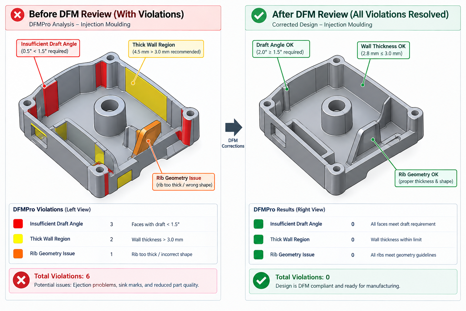
A housing had been designed by an engineer who understood enclosures well. It had good snap-fit latches, correct wall clearances for the PCB inside, adequate rib structure for the drop test, and a textured grip area the product team liked. What it also had, discovered only after tooling was cut, was a 4.8mm wall directly behind a snap-fit boss, unflagged internal undercuts around a USB port, and zero draft on the grip texture.
The molder called with an itemised problem list. The undercuts needed side actions that weren’t in the original tool quote. The thick boss caused a visible sink mark the product team rejected immediately. The textured surface with no draft was tearing on ejection.
Quick answer: The costliest injection molding design mistakes are non-uniform wall thickness, insufficient draft angle, sharp internal corners, unplanned undercuts, and boss or rib walls too close to the nominal wall thickness. All of them are avoidable at the CAD stage with knowledge that costs nothing to apply, and all of them become expensive, sometimes very expensive, once tooling has already been cut.
Three separate design issues, three separate remedies, each avoidable in CAD. The tool rework, delayed launch, and first-shot rejection cost the programme significantly more than the original tooling budget, and all of it traced back to design decisions made without a working understanding of how plastic flows, how moulds open, and what happens to a part between injection and ejection.
The 12 Most Costly Injection Molding Design Mistakes
Each mistake below is a CAD decision with direct consequences at the tool shop, on the injection press, or in the quality inspection booth. All are avoidable at the design stage.
#
Mistake
Root Cause
Typical Cost Impact
Fix
1
Non-uniform wall thickness
Hollowing a solid CAD model without checking resulting variation
Sink marks, warping, longer cycle time; scrap 10-30% on first shots
Keep variation within 10-15% of nominal throughout
2
Insufficient draft angle
Draft added as an afterthought, not designed in
Part sticks; drag marks; ejector pin stress and tool damage
Typical range +/-0.1 to 0.25mm; tighter may not be achievable
The single most important habit: run a draft analysis before releasing any drawing. Most CAD packages colour-code every face relative to a specified pull direction, green for adequate draft, red for insufficient or negative draft. It takes two minutes and catches problems that cost thousands of dollars per face and weeks of delay once tooling is cut.
Mistakes 1 and 2: Non-Uniform and Wrong Wall Thickness
Wall thickness is the single design parameter that most directly controls whether a moulded part looks acceptable, holds its shape, and produces at the assumed cycle time. Get it right and the mould fills evenly, cools uniformly, and ejects cleanly. Get it wrong and the problems cascade: thick sections cool slower than thin ones, so thin sections solidify first while the thick sections pull inward as they cool, creating visible sink marks and internal voids. Severe variation warps the entire part out of flat.
The target isn’t a specific thickness but a specific relationship between walls, following the process fundamentals documented in the Rosato Injection Molding Handbook: keep variation within roughly ten to fifteen percent of nominal throughout the part. A part with a 2.0mm nominal wall shouldn’t have regions thicker than 2.3mm or thinner than 1.7mm without a gradual transition. Where a thick section is unavoidable, taper into it over a distance of at least three times the thickness difference.
Resin Family
Min Wall (mm)
Typical Nominal (mm)
Max Practical Wall (mm)
Key Notes
ABS
1.2
1.5-3.0
4.5
Versatile, forgiving flow; avoid exceeding 3mm without gas assist
Polycarbonate (PC)
1.0
1.5-4.5
6.0
Higher flow resistance; thick walls fill reliably but cycle time is long
PC/ABS blend
1.2
1.5-3.5
5.0
Popular for electronics enclosures; easier than pure PC
Nylon (PA6, PA66)
0.8
1.5-3.0
4.0
Absorbs moisture; design to nominal dry dimension
Polypropylene (PP)
0.8
1.5-3.0
3.5
High shrinkage (1.5-2.0%); excellent for living hinges
Acetal/Delrin (POM)
0.8
1.5-3.0
3.0
Excellent dimensional stability; good for precision gears
PEEK
0.5
1.0-2.5
3.5
Very high processing temperature; expensive resin and process
HDPE
1.0
2.0-4.0
6.0
High shrinkage; waxy surface complicates bonding and painting
PETG
0.8
1.5-3.0
4.0
Good clarity; lower impact resistance than PC
Liquid Silicone Rubber
0.3
0.6-2.5
6.0
Two-component thermoset; excellent for seals, soft-touch grips
How the Solidification Sequence Governs Sink Marks
The mould is cold. The injected plastic is hot. Thin sections next to the cool steel lose heat quickly and solidify into a rigid skin. Thick sections take longer. As a thick section keeps cooling and shrinking after its skin has solidified, the still-soft interior gets pulled inward, and since the far skin is already rigid, the only surface that can move is the opposite face of the thin section adjacent to the thick one. That face dimples inward, producing the sink mark that appears on the cosmetic surface directly opposite the rib or boss.
This is why rib and boss thickness rules are expressed as ratios to the adjacent wall, not absolute values. A 1.5mm rib base next to a 3mm wall, at fifty percent, follows the rule. The same 1.5mm base next to a 1.0mm wall, at one hundred fifty percent, violates it by creating exactly the local thickness excess the rule exists to avoid. Track the ratio, not the dimension alone.
Mistake 2: No Draft Angle on Vertical Walls
When a mould opens, the part has to slide off the core without the walls dragging against the steel. Without draft, the part grips the core tightly as it cools and shrinks onto it, forcing the ejector pins to push it off. The result is drag marks, distortion from uneven ejector loading, and in the worst case a part that sticks entirely, destroying surface finish and risking broken ejector pins.
Draft doesn’t need to be large. On a smooth surface, one degree per side is typically adequate for clean ejection. The fix is applying the right taper before the drawing goes to the mould maker, since draft affects tool steel geometry, parting line position, and ejection layout. Asking for draft after the cavity and core are already machined means re-machining steel already cut to size, expensive and sometimes impossible without scrapping the insert.
Textured Surfaces Need More Draft Than You’d Expect
A smooth surface with one degree of draft ejects cleanly. The same surface with a leather-grain texture and the same one degree won’t. Texture creates physical interlocking with the tool steel, so the part has to tear away rather than slide cleanly, damaging the texture. The standard rule of thumb is one degree of additional draft for every 0.025mm of texture depth, so a leather grain at 0.075mm needs three additional degrees, four degrees total minimum. A heavy texture at 0.150mm needs six additional degrees beyond base draft.
Mistakes 4 and 10: Undercuts and Side Actions
An undercut is any feature preventing the part from being pulled straight out of the mould in the opening direction. Sideways-facing snap-fit hooks, holes on vertical walls, internal threads, wrap-around lips: all trap the part if the mould tries to open in a straight line. The solutions, slides, lifters, collapsible cores, are proven mechanisms used on millions of parts every year, but each adds cost, tool complexity, lead time, and ongoing maintenance considerations.
Undercut Type
Tooling Solution
Cost Premium
Lead Time Impact
When to Accept vs. Redesign
External undercut (lip, sideways hook)
Side action (slide)
+20-35% tooling cost
+2-4 weeks
Accept if function is genuinely required; redesign to a hinged snap if possible
Internal undercut (thread, groove)
Internal lifter or collapsible core
+25-50% tooling cost
+3-6 weeks
Consider a threaded insert or two-piece design before committing
Shallow undercut, flexible material
Forced ejection (stripped over)
No premium
No impact
Accept if material flexes without tearing; typically under 0.5mm depth
Through-hole perpendicular to draw
Simple core pin
No premium
No impact
Always prefer over a blind hole where function allows
Hole on a side face (parallel to parting line)
Side core or split cavity
+10-20% tooling cost
+1-2 weeks
Accept when genuinely functional; verify parting line flash is acceptable
How to Spot an Undercut Before the Drawing Goes Out
Set the pull direction in CAD and run draft analysis, which flags any negative-draft faces as potential undercuts. Sideways-facing faces relative to the pull direction are the most common source. A hole drilled through a vertical wall is a simple example: the core pin forming it runs perpendicular to the pull direction, trapping the surrounding steel unless a slide is provided.
Before budgeting for a side action, ask whether the feature causing it can be moved or redesigned. A sideways-facing snap hook can sometimes become a cantilevered latch that flexes in the pull direction, eliminating the undercut entirely. A hole on a vertical side wall can sometimes move to the parting surface, becoming a through-feature both halves of the tool form, needing no slide. These redesigns take minutes in CAD and save thousands in tooling cost.
Mistakes 7 and 8: Gate Location and Weld Lines
Gate location, where plastic enters the cavity, is one of the most consequential decisions in mould design, and one many designers leave entirely to the mould maker without guidance. That’s a missed opportunity. The design engineer knows which surfaces are cosmetic and cannot show a gate mark, and which features are structural and shouldn’t have weld lines running through them. The mould maker knows injection molding but doesn’t know which is which unless told. Gate location should be a conversation during design, not a surprise after the tool is built.
Gate Type
Appearance
Weld Line Risk
Best For
Avoid When
Edge gate (tab)
Visible stub on parting line; needs degating
Low for simple parts; higher with multiple features
Simple flat parts, prototype tooling
Cosmetic surfaces on the parting line edge
Submarine (tunnel) gate
Auto-degated, small dimple below parting surface
Moderate
High-volume production, labour savings
Brittle resins that crack at the shear point
Pin point gate (3-plate)
Small round mark, auto-degated
Low; positionable away from critical areas
Multi-cavity tools, specific face gating
Large parts with high flow resistance
Hot tip gate
Small vestige only; no cold runner waste
Low, precisely controlled
High-volume, multi-cavity balanced filling
Low-volume runs; heat-sensitive resins
Fan gate
Wide, shallow, visible at parting edge
Very low; distributes flow evenly
Flat sheet-like parts, optical components
Cosmetic surfaces along the gated edge
Valve gate (hot runner)
No or minimal vestige
Low, controllable via timing
Cosmetic surfaces; sequential fill control
High complexity/cost; not for low-volume tools
Weld Lines: Where They Come From and Why They Matter
A weld line forms wherever two flow fronts of molten plastic meet and fuse during filling. Every hole in a moulded part creates one downstream of it, since flow splits around the hole and rejoins on the far side. A part with four holes has at least four potential weld lines. Their location relative to structural loads and cosmetic surfaces is set by gate placement and flow path geometry, and moving the gate can move the weld lines without changing the part’s functional geometry.
Weld lines are mechanically weaker than the surrounding material because the two flow fronts have cooled slightly by the time they meet, and molecular chains and glass fibres (in filled resins) orient parallel to the weld line rather than across it. In unfilled amorphous plastics like ABS, strength reduction might be ten to twenty percent. In glass-filled semi-crystalline plastics like PA66 GF30, it can reach fifty percent, since the fibres that carry load in the base material leave the weld line essentially unreinforced. A weld line running through the root of a snap-fit latch or a screw hole edge is designed to fail there under repeated loading.
Mistakes 5 and 6: Bosses and Ribs That Cause Sink Marks
Bosses and ribs account for more sink mark problems than any other feature type, since both need local material thickness to function, and local thickness excess is exactly what causes sink marks. The rules are simple and widely published, but frequently violated by an instinct to make the boss wall thicker for strength or the rib taller and thicker for stiffness, both of which push directly toward the sink mark the rule exists to prevent.
The Boss Wall Rule
A screw boss needs enough wall thickness to resist hoop stress from screw insertion without cracking, and enough depth for adequate thread engagement. That functional wall thickness is approximately sixty percent of the adjacent nominal wall, providing adequate strength for normal self-tapping screw torque without visible sink marks.
When a designer increases the boss wall beyond sixty to seventy-five percent, the local thickness increase becomes large enough that differential cooling pulls the opposite face inward, producing a visible circular sink mark on the cosmetic surface. The fix once the mould already exists is either texturing the cosmetic surface to hide it or reworking the boss geometry in the tool, both costing money the sixty percent rule would have avoided. Adding a gusset rib from the boss to the nearest structural wall satisfies both the structural requirement and the sink mark rule simultaneously.
The Rib Thickness Rule
Ribs add stiffness without the wall thickness that would increase cooling time, weight, and sink mark risk. But a rib is itself a local thickness increase where it meets the wall, and if the rib base is too thick relative to the wall, it creates exactly the local thick section it was supposed to avoid. The rule: rib base should be fifty to sixty percent of the adjacent nominal wall. A 2mm nominal wall should have ribs no more than 1.0 to 1.2mm thick at the base.
When a designer specifies a rib at seventy-five or a hundred percent of wall thickness for extra structural confidence, the rib creates a local thickness the molding process faithfully converts into a sink mark opposite the rib junction. The fix isn’t a thicker rib, it’s more ribs, each following the fifty to sixty percent rule, distributed over the area needing stiffness. Multiple thin ribs outperform a single thick rib in structural efficiency, sink mark avoidance, and material usage.
Worked Examples
The consumer electronics housing: A mould maker’s pre-tooling review flagged three issues: a 5mm wall behind a snap-fit boss where the designer had added material for strength, a USB port opening on a side wall creating an internal undercut requiring a lifter, and a textured grip area specified with only one degree of draft against a 0.08mm texture depth.
The boss wall was reduced to 1.8mm, sixty percent of the 3mm nominal wall adjacent to it, with a gusset rib added to the nearest internal rib for the structural connection the extra material had been trying to provide. The USB port was relocated so its axis ran parallel to the mould pull direction, converting the undercut into a simple through-feature formed by a core pin, a 4mm position shift the product team accepted after an ergonomics check. The textured faces were redesigned with four degrees of draft, one base plus three for the texture depth.
The tooling was cut to the revised design without any of the three original issues. First shots showed no sink marks, no ejection damage, clean texture release, and matched the original quote. The two days of CAD work prevented what the mould maker estimated would have been a three-to-four-week rework programme costing thirty-five percent of the original tool budget.
The automotive interior component with weld line failures: A trim panel with two mounting holes was gated at the centre of the top edge, sending flow symmetrically toward mounting holes on either side. The flow fronts that split around each hole rejoined directly in line with the screw thread pull-out direction, the axis of highest stress in service. The panel was failing at forty percent of target pull-out force, with clean, planar failure surfaces, the classic morphology of a weld line fracture.
The resin was PA66 GF30, where weld line strength can drop to forty to fifty percent of base material strength. Moving the gate to one end of the panel sent a single flow front across it, still splitting around each hole but rejoining at angles roughly perpendicular to the panel face rather than aligned with the pull-out direction, and the shorter flow path to the far hole reduced the temperature drop before rejoining, improving fusion. Pull-out results improved to ninety-two percent of target, meeting spec, from a runner-only tool modification completed in two days with no cavity or core rework needed.
Frequently Asked Questions
What is the most common injection molding design mistake? Non-uniform wall thickness, and the one with the most visible consequences, since the sink marks it causes show up on cosmetic surfaces where every customer and quality inspector can see them. It’s also the mistake most common among engineers experienced with machined parts, where a thick section just takes longer to cut rather than cooling differently and producing surface defects.
How much draft angle do injection moulded parts actually need? One degree per side is the practical minimum for smooth surfaces, with two degrees giving comfortable margin. For textured surfaces, add roughly one additional degree per 0.025mm of texture depth beyond the base one degree. A light orange-peel texture at 0.025mm needs about two degrees total; a leather grain at 0.075mm needs about four; a heavy tactile texture at 0.15mm may need six or more.
Can I get away without draft angle if I use a good ejection system? Not reliably. Stripper plates, air blast, and heavy ejector pin layouts can push a part off a zero-draft surface, but that force transmits through the part, distorting it or leaving ejector pin marks. For production tooling where appearance and consistency matter, no ejection system reliably substitutes for adequate draft.
What is a weld line and does it always need to be avoided? A weld line is the seam where two flow fronts of molten plastic meet and fuse during filling. They form wherever flow splits and rejoins, downstream of every hole, protrusion, and obstacle, and can’t be eliminated from parts with multiple flow-splitting features. What matters is location and load: a weld line on a hidden, non-structural surface is typically fine, while one through a snap-fit latch root or a mounting boss in glass-filled nylon is a real structural risk.
How tight a tolerance can injection molding actually hold? Typical production parts hold +/- 0.1 to 0.25mm on linear dimensions. Down to +/- 0.05mm is achievable on small parts with controlled process conditions, high-quality tooling, and predictable-shrinkage resins, but needs careful monitoring. Tighter than +/- 0.05mm generally requires secondary operations like machining on specific surfaces. Semi-crystalline resins (nylon, PP) shrink more and less predictably than amorphous resins (ABS, PC).
When should I use a hot runner instead of a cold runner? Hot runners eliminate the cold runner that would otherwise be ejected and scrapped or recycled each cycle, saving material cost and allowing faster cycle times. The manifold itself adds two thousand to twenty thousand dollars to tooling cost depending on complexity, recovered through material and cycle time savings over the production run. This makes economic sense above roughly fifty thousand parts per year for moderate-cost resins, lower for expensive engineering resins like PEEK, and doesn’t make sense for prototype or low-volume tools.
Key Takeaways
The twelve mistakes in this article aren’t exotic edge cases. They’re the items that generate the most tool rework, the most first-shot rejection, and the most programme delays across consumer electronics, automotive, medical, and industrial moulded products. Nearly all of them are avoidable at the CAD stage by an engineer who knows what to look for, and free to fix while the part is still on screen.
The housing story at the start of this article wasn’t a failure of engineering skill. It was a failure of knowledge applied at the right time. Every one of the three problems the mould maker called about has a straightforward CAD fix that takes minutes. The same fix in tooling takes days to weeks and costs real money. Run the draft analysis on every moulded part before the drawing is released. Check every boss and rib against the sixty and fifty percent wall ratio rules.
Walk the pull direction and flag every trapped face. Agree gate location with the mould maker before the tool is designed, not after. These habits are inexpensive in CAD and genuinely expensive to substitute for afterward.
An engineer spent two hours on a Friday afternoon drawing a bracket that looked clean, was correctly dimensioned, and had all the right tolerances. The pocket in the center had sharp 90-degree internal corners because it needed to clear a mating component. One wall was 0.8mm thick because the overall envelope was tight.
The drawing went out for quoting Monday morning. By Tuesday afternoon the shop called back: they could make the bracket, but the sharp corners needed EDM after milling, and the thin wall needed a slow, dedicated setup to cut without chatter. The price reflected both. What looked like a straightforward bracket had become a two-operation part with a lead time measured in weeks, and procurement pushed back on the number.
Quick answer: CNC machining can produce very complex shapes, tight tolerances, and excellent surface finishes, but it can’t do anything a spinning cylindrical tool physically cannot reach. Internal corner radii must match a real end mill radius, wall thickness needs enough rigidity to resist cutting force, and every extra machine setup adds 20 to 40 percent to cost. Designing around these physical constraints from the start, not after a shop quote comes back, is what separates a cheap, fast part from an expensive, slow one with identical function.
None of what the shop said was wrong. The corners really did need EDM, and the wall really did need special process planning. The problem wasn’t in the drawing. It was in the design choices that produced it, made by an engineer who understood the bracket’s structural requirements well but hadn’t built the habit of thinking about what a cutting tool can and cannot reach.
Why CNC Has Design Constraints At All
Every CNC constraint traces back to the same source: the cutting tool is a solid body that must physically reach the feature being cut, and its geometry determines what shapes it can produce. An end mill is a cylinder with cutting edges. When it plunges into a pocket and sweeps the perimeter, it leaves a radius at every internal corner equal to its own radius. That’s not a limitation of machine accuracy or operator skill. It’s a geometric consequence of the tool being round. The only ways around it are a smaller tool (slower, more fragile), EDM (spark erosion instead of a spinning tool), or a design that doesn’t call for a sharp corner there.
Understanding this changes how you approach feature design. The question stops being “what shape do I want here” and becomes “what shape can a tool produce here, and is that compatible with what I actually need.” For most brackets, housings, and structural components, the answer is a straightforward yes once the design adapts. Cases where the functional requirement genuinely conflicts with what a cutting tool can reach are actually rare, and almost always better solved by reconsidering the feature geometry than by accepting the cost of a workaround.
The Three Axes and What They Limit
Most CNC machining centres operate in three axes: X, Y, and Z. The tool reaches any point on the top surface and any vertical surface relative to the current setup. What it can’t reach without repositioning the workpiece are features on other faces, undercuts hidden behind an overhang, and surfaces sloped outside the range of vertical tool motion.
This is why setup count is such an important cost driver. Every time the workpiece is removed, flipped, and re-fixtured, the machine stops producing chips. Repositioning takes time, and re-fixturing introduces a small but real alignment uncertainty that accumulates across the part’s critical dimensions. Reducing a part from four setups to two doesn’t just roughly halve machining time; it also improves positional accuracy between features previously cut in separate setups.
Five-axis machining extends this by tilting or rotating the workpiece relative to the linear axes, reaching compound-angle surfaces and some undercuts in a single setup. It’s genuinely powerful for complex aerospace and medical components, but it costs more per hour, needs more sophisticated programming, and isn’t available at every shop. Commit to a five-axis requirement only after three-axis approaches have genuinely been exhausted, since the pool of shops that can bid narrows and the price rises noticeably once five-axis is a requirement.
CNC Feature Design Rules: The Reference Table
These eight rules are the ones that show up most often in shop feedback, worth checking on every drawing before it goes out for quoting.
Feature
Rule / Guideline
Why It Exists
What Happens If Violated
Internal corner radius (pocket)
Match standard end mill radii: 0.5, 1.0, 1.5, 2.0, 3.0, 4.0, 6.0, 8.0, 10.0mm
End mills are cylindrical, leaving a radius equal to their own
Custom micro-tooling or EDM secondary operation needed
Pocket depth-to-width ratio
Max 4:1 for standard tooling; up to 6:1 with long-reach tooling
Deep narrow pockets need long, thin tools that deflect and chatter
Dimensional error, poor finish, shortened tool life, possible breakage
Hole depth-to-diameter
Through holes: no practical limit. Blind: 3:1 max standard; 5:1 with extended-reach drills
Deep narrow holes need extensions that deflect; chip evacuation is difficult
Shallower threads strip under preload; deeper adds time with no gain
Thread strip-out under torque, especially in softer materials
Wall thickness (milled pocket)
0.5mm minimum rigid materials, short feature height; 1.0mm practical general minimum
Thin walls deflect under cutting force, causing chatter and inaccuracy
Wall bows inward at mid-height, poor finish, out-of-tolerance
Boss/protrusion height
Max 4-5x base diameter for a standard end mill
Tall thin protrusions vibrate and deflect away from the tool
Poor finish, dimensional error, possible feature fracture
Counterbore vs. screw size
Diameter = head diameter + 0.5-1.0mm clearance; depth = head height + 0.2mm
Must clear the fastener head for correct seating
Head protrudes above surface, or contacts bore walls
Chamfers vs. fillets
Chamfers at 45° for standard tooling; fillets need a radius end mill
Chamfers use angled tools; fillets need a ball-nose or radius cutter
A 1mm fillet on every edge triggers a slow finishing pass on all of them
Internal Corners: The Rule That Catches the Most Engineers
The internal corner radius rule is probably the most frequently violated rule in CNC machining, not because it’s complicated but because it’s easy to forget while focused on functional geometry. On a CAD screen, a pocket with sharp 90-degree internal corners looks perfectly clean and buildable. The machinist’s eye sees a feature that requires either a fragile micro-tool that cuts slowly and breaks often, or a standard end mill followed by a secondary EDM operation.
The fix is almost always free in CAD and costs nothing in the part’s function. If the corner radius needs to clear a mating component with a sharp corner, add a corner relief in the mating part instead of requiring a sharp corner in the pocket. If the radius is simply unconstrained, size it to the nearest standard end mill and the issue disappears. A 6mm internal radius lets any end mill up to 12mm diameter finish the corners, giving the shop far more flexibility than a 1mm radius would.
Below about 1mm internal radius, you’re in micro-machining territory. Tools at this scale are fragile, cut slowly, and need spindles running 20,000 to 50,000 RPM to maintain reasonable surface speeds. Cost per feature rises sharply, breakage risk is meaningful, and the range of shops that can produce it reliably narrows. This isn’t to say micro-machining is never appropriate, medical devices, optical mounts, and precision instruments genuinely need it sometimes, but it should be a deliberate choice against a known requirement, not an accidental consequence of a sharp corner in a standard bracket.
Tolerances and Surface Finish: Only as Tight as the Function Needs
One of the most reliable ways to add cost without adding value is specifying tolerances tighter than the application requires. This happens for a few common reasons: CAD title block defaults that carry a tolerance tighter than most features need, dimensions copied from a previous design, and a conservative instinct that tighter is always safer. None of those reasons are wrong in intent, but they all lead to a shop running additional operations or more extensive inspection to hit a number that serves no purpose in the finished assembly.
The discipline worth applying: for every toleranced dimension, ask what actually breaks if the tolerance were twice as loose. If the answer is genuinely nothing, the tolerance is tighter than needed. For most non-mating, non-locating dimensions on a structural part, a general tolerance of +/- 0.125mm to +/- 0.25mm is perfectly adequate, matching the standard tolerance classes documented in Machinery’s Handbook, and achievable without any special process consideration.
Feature Type
Standard Tolerance
Achievable Tighter
Added Operation for Tighter
General machined dimension
+/- 0.125 to 0.250mm
+/- 0.05mm with careful setup
None standard; extra fixturing for +/-0.05
Drilled hole diameter
+0.10/-0.00 (drilled nominal)
+/- 0.025mm (reamed)
Reaming adds one tool change, one pass
Bored hole diameter
+/- 0.025 to 0.050mm
+/- 0.005-0.010mm
Fine or jig boring; climate control
Tapped thread
ISO 6H (medium fit)
ISO 5H or 4H (close fit)
Machine tapping vs. hand; gauge verification
Flatness (milled)
0.05-0.10mm over 100mm
0.01-0.02mm over 100mm
Grinding or precision milling with temp stabilisation
Surface Finish Is a Secondary Operation, Not a Milling Setting
Surface finish finer than Ra 0.8 micron typically can’t be achieved by milling alone regardless of cutting parameters. Ra 0.4 micron or better needs a secondary process, grinding, lapping, or honing, each a separate production step with its own setup and cycle time. Specifying Ra 0.4 on a surface that serves no sealing, sliding, or tribological function adds an entire secondary operation for no functional benefit.
The practical approach: specify surface finish only where it matters functionally, and use the loosest specification that still meets the requirement. A sealing face needs smoothness for the seal to seat without leaking. A sliding contact needs a finish appropriate for its bearing pressure. Everything else can stay as-machined, typically Ra 1.6 to 3.2 micron, which costs nothing extra since it’s what standard milling produces without additional operations.
Material Machinability: How Material Choice Affects Cost
Material choice is one of the most consequential machining cost decisions, typically locked in early, before any features are designed. A designer who understands machinability characteristics upfront can sometimes cut machining cost by thirty to fifty percent with a material choice that still satisfies engineering requirements.
Material
Machinability Rating
Key Consideration
Tool Life Impact
Aluminium (6061, 7075)
Excellent: 200-300% of free-cutting steel
Long, stringy chips need chip-breaker geometry
Very long tool life; carbide and HSS both work well
Mild steel (1018, 1020)
Good: 70-80%
Free-machining grades (1215, 12L14) are significantly easier
Moderate; carbide preferred for production runs
Stainless steel (304, 316)
Difficult: 40-50%; work-hardening is the challenge
Must cut continuously; carbide tooling mandatory
Short tool life; 303 free-machining much easier if allowed
For most structural steels, free-machining grades exist that are substantially easier and cheaper to machine than standard equivalents, with only modest property compromises. 1018 is the workhorse structural grade with good strength and weldability. 1215, a resulfurized free-machining grade, machines at roughly twice the speed with better surface finish and longer tool life. If the application doesn’t need welding, heat treatment, or 1018’s slightly higher strength, switching to 1215 often halves machining cost for no functional penalty.
The same trade-off exists in stainless: 303 machines three to four times faster than 304, with better finish and much longer tool life, at the cost of weldability and slightly lower corrosion resistance in some environments. A lot of engineers default to 304 simply because it’s the most widely specified grade, without checking whether the application actually needs what 304 provides over 303, and that default carries a real cost penalty on every unit produced.
Setups and Fixturing: Designing for How the Part Sits in the Machine
Every time a machinist repositions a part, the clock runs but no chips get made. Fixturing, alignment, and probing each take time, and setup count is one of the clearest predictors of cost. A part needing three setups doesn’t simply cost 50 percent more than one needing two. The operator also has to re-establish the datum reference each time, small alignment errors accumulate between features cut in different setups, and a custom fixture may be needed if the geometry doesn’t lend itself to standard workholding.
Design for Standard Workholding
Standard workholding means a machine vise, a collet chuck, or toe clamps on a fixture plate. Parts with flat, parallel reference surfaces and enough clearance for vise jaws to grip without interfering with the cut features are the cheapest to set up and the least likely to trigger a call about needing a custom fixture. Round or organically shaped parts, or ones with features that conflict with standard vise jaw positions, need a custom fixture or an angled setup that introduces risk.
The practical habits: keep at least two opposite faces flat and parallel as datum surfaces for vise workholding, make sure features needed in each setup are accessible from the top without vise jaws blocking the tool path, and avoid features requiring the part to be fixtured at an angle, since angle plates and tilted fixtures add cost and setup time.
The 2+2+2 Setup Rule for Rectangular Parts
Think of a rectangular part’s six faces as three pairs: top and bottom, front and back, left and right. A well-designed three-axis part should have all its features accessible from at most three of those faces. Top-face features get cut in setup one, front or back face in setup two with the part stood on end, and a side face in setup three. That’s the practical limit of efficient three-axis machining without a rotary fourth axis or a five-axis machine, and designing within it keeps the part accessible to the widest pool of suppliers.
CNC Cost Drivers: What Makes a Part Expensive
Not all cost drivers are equally within a designer’s control, and not all carry equal weight.
Cost Driver
Relative Impact
Design Changes That Reduce It
Red Flags in a Drawing
Number of setups
High: 20-40% per additional orientation
Design features on as few faces as possible
Features requiring more than one flip; holes on 5-6 faces
Tight tolerances
High, non-linear: 1.5-6x cost per tighter class
Specify no tighter than function demands
Tight tolerances on cosmetic features; blanket +/-0.025mm title block
Deep narrow pockets
Medium-High
Widen pockets for a stiffer tool; step the depth down
Depth-to-width above 4:1; narrow full-depth slots
Small internal corner radii
Medium
Match standard end mill sizes
Internal corners under 1.0mm without micro-machining need
Custom tooling or operations
Very High: weeks of lead time, high cost
Design to standard tool sizes and thread forms
Non-standard thread forms; radii matching no available tool
Surface finish requirements
Medium
Specify finish only where functionally needed
Ra 0.4-0.8 on surfaces with no sealing/bearing/mating function
Material removal volume
Medium
Remove only what the design needs
50mm billet machined down to a 3mm plate
Part size vs. machine capacity
Low-Medium
Split oversized parts where the design allows
Parts approaching a 600-800mm three-axis envelope
The Setup Count Problem Is Easy to Underestimate
Setup count is the cost driver most frequently underestimated by engineers without shop floor experience. A design requiring five setups doesn’t just add four extra repositionings’ worth of time. It also shrinks the pool of shops that can run the part economically, since tying up a machining centre for five operations is only profitable at certain volumes and price points. An engineer who reconsiders a four-setup layout and finds a way to do it in two hasn’t just cut unit cost; they’ve opened the part to a wider range of competitive bids, which often drives cost down further.
Worked Examples
The pump housing with EDM corners: A pump housing had a rectangular internal cavity for a sliding valve with square cross-section corners, so the designer specified a matching square cavity with zero-radius corners on all four internal walls. The sharp corners required EDM after milling, adding roughly 60 percent to machining cost and extending lead time from five to twelve days.
The redesign kept the valve body’s functional cross-section but added 2mm corner reliefs to the valve, matching the radius a 4mm end mill would leave in the housing cavity. The cavity became fully machinable with a standard end mill in one operation, and the valve still slid correctly since the reliefs didn’t interfere with any sealing or guidance surface. The EDM step was eliminated entirely, machining cost dropped roughly 45 percent, and lead time returned to five days, all from an hour of CAD work with zero impact on function.
The instrument bracket with unnecessary surface finish: An optical instrument bracket carried a Ra 0.4 micron finish requirement on all machined surfaces, inherited from the finish standard of the optical instrument it mounted. The bracket itself was purely structural, none of its surfaces were optical, sealing, or sliding contacts. That blanket finish requirement meant grinding every face as a secondary operation, accounting for sixty percent of total machining cost.
The revision set structural faces to Ra 1.6 micron as-milled, keeping Ra 0.4 micron only on the two precision datum surfaces where the instrument actually seated. Grinding dropped from six faces to two. Machining cost fell roughly 40 percent and lead time shortened from eight days to four, with zero change to the instrument’s optical performance since the surfaces that actually mattered kept their required finish.
Frequently Asked Questions
What is the minimum internal corner radius I should design for? The practical floor is set by the smallest standard end mill your shop carries, typically 1mm diameter for a 0.5mm corner radius, but that size is fragile and slow. A more practical minimum for typical work is 1.5mm to 2.0mm, matching common, robust 3mm and 4mm tools. Designing to 3mm or 6mm gives even more tool selection flexibility, usually translating to faster cycle times and lower cost. Choose the largest radius the design will tolerate functionally, matched to a standard end mill size.
How many setups should I aim for? One setup is ideal wherever function allows it. Two is the practical target for most rectangular parts. Three is the practical limit for standard three-axis equipment without a rotary axis. Once a part needs four or more, cost rises substantially and the pool of shops that can run it economically narrows. If a design is heading toward four or more setups, ask whether features can be relocated or consolidated, or whether five-axis machining would bring the setup count down to one or two and improve the economics for your volume.
Does material choice really affect machining cost that much? Yes, significantly. The difference between 303 stainless (free-machining) and 316 for the same part can be a factor of two to three in cycle time alone, with tool wear compounding it further. The difference between 6061 aluminium and Ti-6Al-4V for a structurally equivalent part can run five to ten times in total machining cost. For meaningful production volumes, machinability deserves the same attention as structural material selection, since there are often two or three material options within a given structural requirement with very different machinability profiles.
When should I use a chamfer instead of a fillet on an external edge? Use a chamfer whenever the purpose is deburring, lead-in for assembly, or a cosmetic break, and a fillet isn’t structurally required. A 45-degree chamfer is cut in a single fast pass. An external fillet needs a ball-nose or radius end mill making a slower finishing pass around every edge that carries the callout. On a part with many external edges, specifying fillets everywhere can add a full finishing operation. Reserve fillets for features where the radius is functionally required, like a fatigue-critical wall-to-floor transition, or a load-distributing contact surface.
Why do tighter tolerances cost so much more? Because tighter tolerances usually trigger a step change in process rather than a smooth increase in care. A hole at a standard drilling tolerance needs one operation. The same hole at +/-0.025mm needs reaming: an additional tool, an additional pass, additional inspection. Flatness at 0.05mm over 100mm might be achievable with careful milling; 0.005mm needs grinding in a temperature-controlled environment. Each tighter step tends to require an additional operation or a different process entirely, which is why tolerance cost looks like a series of jumps rather than a smooth curve.
What’s the maximum depth-to-width ratio for a CNC pocket? The standard guideline is 4:1 for pockets machined with a standard-length end mill. At that ratio, the tool already experiences meaningful deflection under cutting load, affecting finish and accuracy, particularly at the bottom corners. Above 4:1 you need long-reach tooling, which deflects more, cuts more slowly, and costs more. Above 6:1, options are accepting long-reach tooling’s cost, widening the pocket at deeper sections, splitting the part into two conventionally machined pieces, or switching to EDM for the deep sections, which avoids deflection but runs considerably slower than milling.
Key Takeaways
The bracket from the opening example eventually got made, at a higher cost and longer lead time than expected. That’s not the worst outcome, and it’s far from unusual. Most engineers learn these rules from experience, from parts that cost too much, took too long, or generated a call from the shop about a feature the drawing hadn’t accounted for.
The goal is to move that learning earlier, before a drawing goes out, before tooling is committed, while the features are still adjustable in CAD at no cost. These rules aren’t creative constraints on what a part can look like. They’re physical facts about what a spinning cylindrical tool can and cannot do through three or five axes. A designer who has internalised them thinks differently about feature geometry, not less ambitiously, but with a natural awareness of which choices translate directly into cost and lead time.
Run through the reference tables whenever a CNC drawing is close to final. Check internal corner radii against the feature rules. Audit every tight tolerance. Count the setups the current feature layout requires and whether any change would reduce it. Those checks cost minutes in CAD. The problems they catch cost days or weeks and real money once the drawing is at a shop.
A gearbox housing kept failing its final assembly check. Not often, maybe one unit in forty, but often enough to stop the line every shift over a shaft that wouldn’t seat against its retaining ring. Every individual part had passed inspection. Every dimension on every drawing sat within its stated tolerance stack up.
The engineering team spent two weeks chasing a phantom defect before someone laid all five parts in the stack-up out on a bench, added up their tolerances by hand, and found the answer. The design had been toleranced as if the parts would average out around nominal, but nobody had checked what happened if four of the five parts landed near the same edge of their range at once. When that happened, a small but real fraction of the time, the stack came up short by just over a tenth of a millimetre, and the shaft wouldn’t seat.
Quick answer: Tolerance stack-up is the accumulated effect of individual part tolerances on a final assembled dimension. It’s one of the most common ways a product that looks correct on every individual drawing still fails when the parts come together, because no single part is wrong; the problem lives in how several correct tolerances combine. The four standard calculation methods are worst-case, RSS (root sum square), Cpk-adjusted statistical analysis, and Monte Carlo simulation, and choosing between them is a real engineering decision with direct cost and quality consequences.
[Image suggestion 1: An exploded-view diagram of the five-part gearbox axial stack (housing wall, spacer, bearing, shaft shoulder, retaining ring) with dimension callouts and arrows showing the cumulative tolerance chain. Alt text: “Exploded diagram of a five-part gearbox tolerance stack-up showing housing, spacer, bearing, shaft, and retaining ring dimensions”]
What a Tolerance Stack-Up Actually Is
Every dimension on a drawing has a tolerance, a permitted range of variation around nominal. On its own, that tolerance describes how much one feature on one part can vary and still be acceptable. A stack-up happens whenever an assembled dimension, a gap, a clearance, an alignment, depends on more than one of those individually toleranced dimensions adding together. The assembled dimension inherits variation from every contributor in the chain, and a stack-up calculation answers a single question: how much can that final dimension actually vary, given everything feeding into it?
The gearbox chain had five links: housing wall location, spacer thickness, bearing width, shaft shoulder position, and retaining ring thickness. Each tolerance was individually reasonable and individually achievable. None of them was the problem. The problem was that nobody had calculated what all five could produce in the worst case, and the design was sized as though nominal values alone would always be close enough.
This is the trap that catches engineers comfortable with individual part tolerancing but who haven’t built the habit of tracing assembled dimensions back through every contributor. A stack-up isn’t a single calculation done once. It’s a discipline: identify every dimension contributing to a critical assembled feature, decide how those contributions combine, and check the result against what the assembly actually needs. Skip any one of those steps and the calculation, even with correct arithmetic, won’t tell you what you need to know.
Four Ways to Calculate a Stack-Up
There’s more than one accepted way to combine individual tolerances into a predicted range for the final assembled dimension, and the methods don’t agree with each other. Two engineers looking at the same five-part gearbox stack could reach different conclusions about whether the design is safe, depending entirely on which method they used.
Method
Formula (linear stack)
What It Assumes
Resulting Range
When to Use
Worst-case (arithmetic)
T_total = T1+T2+…+Tn
Every dimension simultaneously at its limit, worst combination, every time
Widest possible; guarantees 100% fit but most conservative and expensive
Each dimension varies independently, roughly normal distribution
Typically 40-60% tighter than worst-case for 4+ dimensions
Medium/high volume with statistically stable independent processes
Six Sigma (Cpk-adjusted RSS)
T_total = sqrt(sum((Ti/Cpki)²))
Each input has a known or assumed process capability, not just a tolerance
Tighter or looser than basic RSS depending on real Cpk
Mature processes with historical Cpk data; automotive, medical, aerospace
Monte Carlo simulation
Numerical: thousands of randomized trials
Each input’s actual distribution shape is known or reasonably estimated
Most accurate real-yield representation; handles non-linear stacks
Complex assemblies with 6+ contributors or non-normal distributions
Worst-Case: Simple, Safe, and Often Too Expensive
The worst-case method is the one most engineers learn first because the logic is completely intuitive: add every plus tolerance for the maximum stack, every minus tolerance for the minimum, and you have a guaranteed range covering every physically possible part combination. If the assembly works at both ends of that range, it works no matter what actually gets built. No statistical assumption hides in the background. It’s a hard guarantee.
The cost of that guarantee grows quickly as more dimensions join the chain. In reality, the chance that five independent parts all land at the same tolerance edge simultaneously is vanishingly small, smaller as more parts join the stack. Worst-case tolerancing protects against an outcome that’s real but rare for most production processes. That protection is worth paying for on a safety-critical aerospace joint, and much harder to justify on a cosmetic gap that would be far cheaper to fix with a slightly tighter tolerance somewhere else in the chain.
RSS: Letting Statistics Do the Work
RSS takes a different view of the same problem. Instead of assuming every part lands at its tolerance extreme simultaneously, it assumes each dimension varies independently around its own nominal, the way a real, statistically stable process actually behaves. Most parts come out close to nominal. Fewer land near the limits. The chance that several independent dimensions all land at an extreme together is much lower than the chance that any single one does, and RSS reflects that by combining tolerances as the square root of the sum of squares rather than a simple sum.
The result is almost always tighter than worst-case, often forty to sixty percent tighter once a stack has four or more contributors. That’s exactly why RSS is attractive: it predicts, correctly for processes that actually behave this way, that the assembled result varies less than worst-case suggests. The catch is real: RSS only holds up if the assumption is true. If a contributing process isn’t statistically stable, or if two dimensions in the stack aren’t actually independent because they come from the same tool or fixture, RSS understates the real variation, and a gearbox-style failure becomes a possibility the calculation never warned anyone about.
Cpk-Adjusted Statistical Methods: Bringing Real Process Data In
Basic RSS treats every contributing dimension as if its real variation exactly fills its stated tolerance band. In practice that’s rarely true. A mature, well-controlled process often clusters much more tightly around nominal than the tolerance alone suggests, while a newer process might run close to its limits. Process capability, expressed as Cpk, captures that difference.
Cpk Value
Sigma Level
Defect Rate (PPM)
What It Means
Typical Process Maturity
0.67
2 sigma
~22,750 ppm (2.3%)
Process spread nearly fills the band; frequent defects expected
New or poorly controlled; pilot run before optimisation
1.00
3 sigma
~1,350 ppm
Spread just fits under ideal centring; any drift causes defects
Marginal control; acceptable for low-consequence features
Variation a small fraction of the band; defects effectively eliminated
Six Sigma mature; semiconductor, medical, aerospace critical
Using actual Cpk data instead of a flat industry-default value changes the calculation meaningfully. A dimension running at Cpk = 2.0 barely uses its tolerance band and contributes very little real variation, while one at Cpk = 1.0 fills its band almost completely. A stack-up treating both the same, assuming a uniform Cpk across every contributor, will be wrong in one direction or the other. The only way to know which is to look at the actual process data, following the process capability framework laid out in the AIAG Statistical Process Control reference manual, rather than assume it.
Monte Carlo: When the Maths Gets Too Complicated for a Formula
Worst-case and RSS work cleanly for simple linear chains, but real assemblies aren’t always that simple. Some stack-ups involve trigonometric relationships, angular tolerances combining with linear ones, or contributors whose distribution isn’t close to normal, none of which fits neatly into the RSS formula. Monte Carlo sidesteps the problem entirely: it randomly samples each contributing dimension thousands of times according to its actual or assumed distribution, calculates the resulting assembled dimension for every random combination, and builds a complete picture of the likely outcome from the simulated results directly.
The advantage is that Monte Carlo handles almost any complexity, non-linear relationships, mixed distribution shapes, correlated inputs, without needing a closed-form formula for the specific geometry. The cost is that it requires dedicated tolerance analysis software or custom calculation setup, and the result is only as good as the distribution assumptions fed into it. For complex assemblies with six or more contributing dimensions, or stacks mixing angular and positional tolerances with linear ones, Monte Carlo is usually the most trustworthy method available.
A Worked Calculation: The Gearbox Stack-Up Revisited
Laying out the five contributing dimensions and running each method is exactly the exercise that would have caught the gearbox problem before it reached the assembly line.
CONTRIBUTING DIMENSIONS (mm):
Housing wall to bearing seat: 25.00 +/- 0.10
Spacer thickness: 5.00 +/- 0.05
Bearing width: 12.00 +/- 0.08
Shaft shoulder position: 8.00 +/- 0.06
Retaining ring thickness: 2.00 +/- 0.03
NOMINAL STACK: 25.00 + 5.00 + 12.00 + 8.00 + 2.00 = 52.00 mm
Required clearance for correct seating: 52.00 mm +0.05 / -0.00
METHOD 1: WORST-CASE
T_total = 0.10 + 0.05 + 0.08 + 0.06 + 0.03 = 0.32 mm
Predicted range: 51.68 to 52.32 mm
Against required +0.05/-0.00: EXCEEDS limit in worst case
METHOD 2: RSS (Cpk = 1.33 assumed, normal distribution)
T_total = sqrt(0.10²+0.05²+0.08²+0.06²+0.03²) = sqrt(0.0234) = 0.153 mm
Predicted range: 51.85 to 52.15 mm
Against required +0.05/-0.00: STILL EXCEEDS the +0.05 limit
WHAT THIS REVEALS:
Even the more forgiving RSS prediction (0.153mm) exceeds the
functional requirement (0.05mm). This is not a method problem,
it is a genuine design problem: the individual tolerances are
too loose for the function.
CORRECTIVE ACTION TAKEN:
Bearing width tightened from +/-0.08 to +/-0.03 (tighter-spec bearing)
Housing wall tightened from +/-0.10 to +/-0.05 (reaming vs. as-drilled)
New RSS: sqrt(0.05²+0.05²+0.03²+0.06²+0.03²) = 0.102mm
Still tight vs. +0.05/-0.00 -- requires selective assembly
or further tightening; escalated for design review
Every one of the five original tolerances was perfectly reasonable on its own drawing. None would have raised a flag in an isolated review. It was only adding them together, in the actual functional direction they combine, that revealed the design couldn’t meet its own clearance requirement. That revelation is the entire value of a stack-up calculation.
How Stack-Up Errors Show Up in Real Products
The same underlying problem, accumulated variation across a chain of dimensions, shows up differently depending on what’s being built.
Industry / Product
Example Stack-Up
Consequence
Typical Method Used
Automotive body-in-white
Door gap/flush: panel, hinge, striker, body opening
Visible gaps, wind noise, water leaks, warranty claims
RSS or Six Sigma Cpk-adjusted; Cpk >= 1.33 typical
Why Automotive Panel Gaps Are the Textbook Example
Door gaps and panel flush conditions are among the most visible, most photographed examples of tolerance stack-up in everyday life, because the human eye is extremely sensitive to uneven gaps between adjacent panels. A door gap varying from 4mm at the top to 6mm at the bottom is immediately obvious to a customer, even though both values might individually sit within a reasonable-looking tolerance.
That sensitivity is exactly why automotive OEMs push hard on statistical process control and Cpk targets for body panel dimensions. The stack-up producing a door gap runs through the body structure, hinge, striker, and door panel, and a worst-case approach applied to that whole chain would require individual tolerances so tight the parts would be prohibitively expensive at automotive volumes. The only way to hit both the cosmetic requirement and a sane production cost is statistical tolerancing backed by real, monitored process capability, which is why Cpk targets of 1.33 or higher on body panel dimensions are standard rather than an unusual aspiration.
Common Mistakes That Undermine a Stack-Up Calculation
A stack-up calculation can be arithmetically correct and still mislead, because the maths is only as good as the assumptions and completeness feeding into it.
Mistake
Why It Happens
Consequence
Fix
Mixing worst-case and statistical dimensions without flagging it
Different engineers contribute dimensions without agreeing on a shared method
Result is neither a valid worst-case bound nor a valid statistical estimate
Agree on the method per chain before dimensions are finalised; document it
Leaving out a contributor because it “shouldn’t matter”
Stack diagram built from the drawing without a deliberate walk of every contact
Calculated tolerance is optimistic; real assemblies show more variation
Build the stack from a physical or simulated walk of the actual load path
Treating a bilateral tolerance as one number instead of plus/minus
Quick mental math collapses +/-0.1 into 0.1 without tracking direction
Sign errors that understate or overstate the range, sometimes by 2x
Carry plus and minus contributions separately; use tools that enforce this
Assuming RSS without verifying independence and normal distribution
RSS is the default in most software, applied without checking assumptions
Correlated dimensions (shared tooling/fixture) make RSS understate variation
Identify shared process dependencies first; use Monte Carlo if correlated
Using Cpk = 1.33 for every dimension regardless of real history
It’s the common default and easier than pulling real capability data
Calculated yield is fictional if a process actually runs lower
Pull actual Cpk data wherever it exists; flag assumed values explicitly
Stacking only nominal dimensions and ignoring GD&T
Linear stacks are easier to set up than full GD&T-based stacks
Assemblies fail even when every linear dimension is in tolerance
Include position, perpendicularity, and flatness as contributors
The Independence Assumption Is the One Worth Double-Checking Most
Assuming statistical independence when it doesn’t actually exist is probably the mistake that causes the most damage while being hardest to spot from drawings alone. RSS and Cpk-adjusted methods both depend on each contributing dimension varying independently of the others. That holds reasonably well when each dimension comes from a genuinely separate process, machine, or setup.
It breaks down when two or more dimensions in the same stack are produced on the same fixture, machined in the same setup, or molded in the same cavity, because whatever makes that shared process drift, tool wear, thermal expansion, fixture wear, tends to push those dimensions in a correlated direction rather than randomly and independently. A stack-up treating correlated dimensions as independent understates real variation, sometimes significantly, which is exactly the gap between calculation and reality that produced the gearbox failure. The fix: before defaulting to RSS, ask whether any two contributors share a fixture, a tool, or a process step, and treat those as correlated if they do.
Building Stack-Up Analysis Into the Design Process
The gearbox failure wasn’t caused by a lack of skill. It was caused by the stack-up calculation simply not happening until after parts were already failing on the line. The fix isn’t a better formula, it’s a process change: deciding, as a matter of routine, which assembled dimensions warrant a formal stack-up calculation, and doing it before tooling is committed rather than after a quality problem forces the question.
Identify the critical assembled dimensions first. Walk the assembly and identify every gap, clearance, or alignment that actually matters functionally or cosmetically, deliberately rather than after a failure.
Trace the actual contact chain for each critical dimension. Trace every part, feature, and contact surface that physically contributes, the way the gearbox team eventually did on the bench. This step gets skipped or done from memory more often than any other.
Choose a stack-up method deliberately, and document the choice. Base it on the consequence of failure and the maturity of the contributing processes, and write the decision down.
Calculate before tooling, not after. Run it while the design is still in CAD and individual tolerances can still be adjusted cheaply.
Validate against real measured data once production starts. Compare the actual assembled dimension to the prediction, and use any gap to correct the assumptions feeding future stack-ups.
The minimum question to ask before releasing any assembly drawing: if every contributing dimension landed at the worst end of its tolerance simultaneously, would this still function? If the honest answer is no, and the design is relying on statistics to save it, that reliance needs to be a deliberate, documented decision, not an assumption nobody checked.
Frequently Asked Questions
What is the difference between worst-case and statistical tolerance stack-up? Worst-case adds up every individual tolerance directly, guaranteeing the assembly works for every physically possible part combination, but the predicted range grows quickly as dimensions join the chain, usually demanding tighter and more expensive individual tolerances. RSS assumes each dimension varies independently around nominal and combines tolerances as the square root of the sum of squares, producing a tighter, more realistic range, but only if the dimensions are genuinely independent and statistically stable.
When should I use worst-case instead of RSS for a stack-up? Use worst-case when the consequence of an out-of-tolerance assembly is severe: safety-critical interfaces, low-volume production, or any case where reliable process capability data isn’t available. Use RSS or Cpk-adjusted methods when volume is high enough that the processes are genuinely stable, the consequence of an occasional miss is manageable, and you can support the independence assumption. Many designs mix both: worst-case for the dimensions that matter most, RSS for the rest of the same stack.
What does Cpk actually measure and why does it matter for stack-up? Cpk measures how well a process’s actual output variation fits within the specified tolerance band, accounting for how centred the process is on nominal. A Cpk of 1.33 leaves a comfortable margin, roughly 32 defects per million. A Cpk of 1.0 barely fits the band, roughly 1,350 defects per million, with little margin for drift. Cpk matters because basic RSS assumes every dimension’s variation fills its tolerance band evenly, which is rarely true. Folding in real Cpk data lets the prediction reflect how parts are actually being made.
How many dimensions need to be in a chain before stack-up becomes a real concern? There’s no fixed number; it depends on the size of each tolerance relative to the functional requirement, not just the dimension count. As a practical rule, any assembled dimension built from three or more individually toleranced contributors deserves a deliberate calculation rather than an assumption that nominal values will be close enough. A five-part stack feeding a tight clearance, like the gearbox example, almost always needs one.
Can a tolerance stack-up calculation be wrong even if the arithmetic is correct? Yes. The arithmetic in a worst-case or RSS calculation is simple and rarely the source of error. The calculation goes wrong when the inputs are wrong: a contributor left out because it seemed unimportant, an assumed Cpk that doesn’t match the real process, an independence assumption applied to dimensions that actually share a fixture, or a sign error from collapsing a bilateral tolerance without tracking direction. A stack-up is only as trustworthy as the completeness and accuracy of what feeds into it.
Is Monte Carlo simulation always better than RSS for tolerance analysis? Not always, though it’s more broadly capable. RSS is fast, needs no special software, and gives a perfectly good answer for simple linear stacks with normally distributed, independent inputs, which describes a large share of real-world stack-ups. Monte Carlo earns its extra setup cost for non-linear relationships, non-normal distributions, or enough contributors and complexity that a closed-form RSS formula becomes difficult to set up correctly. For a five-part linear stack like the gearbox example, RSS is entirely adequate; for a complex multi-axis assembly mixing angular, position, and linear tolerances, Monte Carlo is usually more trustworthy.
Key Takeaways
Every individual dimension on every drawing in the gearbox assembly was correct. That’s exactly what makes tolerance stack-up worth taking seriously: it’s one of the few places in engineering where every individual piece of work can be done right and the overall result can still fail, because nobody added the pieces together and checked. The product didn’t fail from a mistake on a drawing. It failed because the relationship between five correct drawings was never examined.
Worst-case, RSS, Cpk-adjusted analysis, and Monte Carlo simulation aren’t competing answers to the same question. They’re different tools suited to different situations, and choosing between them is itself an engineering decision deserving the same deliberate attention as any individual tolerance. They all share the same purpose: turning a collection of individually reasonable tolerances into an honest answer about whether the assembled product will actually work, calculated before tooling is cut, not discovered after parts are already failing on the line.
An injection-moulded enclosure looked fine on screen. Wall thickness ranged from 1.2mm to 4.8mm across the part because the designer hollowed out a solid model without tracking where the resulting walls changed thickness. Nobody caught it in CAD review, since the review checked fit and function, not wall uniformity.
The tooling got cut. First shots showed sink marks over every thick section and a warp across the lid that threw the snap-fit tabs out of alignment by half a millimetre. Fixing it meant reworking tool steel and revalidating fit. The change cost eleven thousand dollars and pushed launch back six weeks.
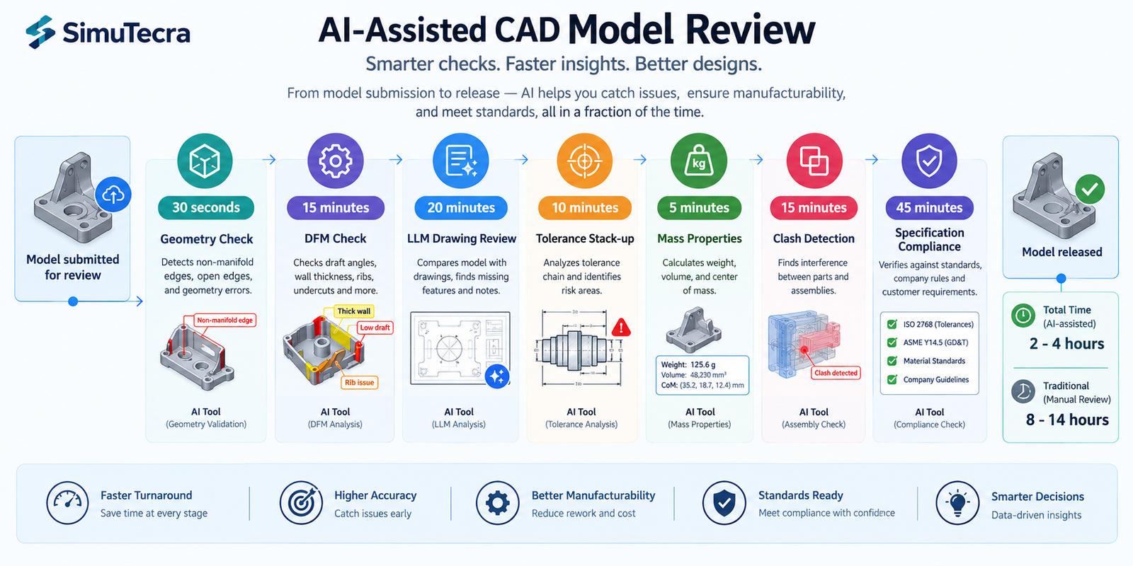
Quick answer:Design for manufacturability (DFM) is the set of process-specific constraints that turn a geometrically correct CAD model into a part that can actually be produced, at target cost, without surprises after tooling is committed. The highest-leverage checks are wall thickness uniformity, draft angles, internal fillet radii, and tolerances specified no tighter than function requires. None of these are engineering skill gaps; they’re a missing systematic check against how the part will actually be made.
This guide covers the four processes most engineers actually work with: injection moulding, CNC machining, sheet metal forming, and assembly. It includes a 20-item checklist with priority ratings, four reference tables with the numbers you need at the CAD stage, and worked examples showing how a DFM review changes a part before it reaches a tool shop.
The 20-Point DFM Checklist
This master checklist spans all four process families and is built to scan quickly during a design review. Critical items cause part failure, tooling damage, or major rework if missed. High items cause significant cost or schedule impact. Medium items are good practice that controls cost without being make-or-break.
Hole diameter-to-depth ratio within process limits
Machining, moulding, casting
Drill wander, tool breakage, incomplete fill
High
6
Avoid undercuts unless side-action tooling is budgeted
Moulding, die casting
Requires slides/lifters; tooling cost +20-50%
Critical
7
Standard fastener sizes and thread specs used
Assembly, machining
Custom fasteners cost 3-10x standard
High
8
Tolerances specified only as tight as needed
Machining, all processes
Cost increases exponentially per tightened tolerance
Critical
9
GD&T datums match assembly and inspection method
Machining, inspection
Unmeasurable tolerances; assembly issues
High
10
Symmetric or self-locating parts
Assembly
Incorrect assembly; warranty and rework cost
High
11
Minimize part count through consolidation
Assembly, all processes
Each part adds time, inventory, failure points
High
12
Avoid dissimilar materials without joining plan
Assembly, welding, bonding
Galvanic corrosion; CTE mismatch failure
Critical
13
Bend radius meets minimum per material/thickness
Sheet metal
Cracking at bend; unpredictable springback
Critical
14
Features kept clear of bend lines (2-3x thickness)
Sheet metal
Distortion near bend; feature tolerance lost
High
15
Machined features accessible without special tooling
CNC machining
Custom fixtures or multiple setups needed
High
16
Parting line positioned to minimize flash
Die casting, sand casting
Excess flash removal labor; cosmetic defects
Medium
17
Weld joint design matches process capability
Welding/fabrication
Poor penetration, distortion, rework
Critical
18
Surface finish specified only where necessary
Machining, finishing
Unnecessary polishing operations add cost
Medium
19
Design supports automated inspection
Quality/inspection
Manual inspection required; slower, less repeatable
Medium
20
Reviewed against supplier’s process capability data
All processes
Design exceeds shop capability; late redesign
Critical
How to use this checklist: Run it at the CAD stage, before any drawing goes out for quoting or tooling. It works best as a joint review between the design engineer and someone with shop-floor or supplier experience, since the reference table numbers are starting points, not universal constants. Every supplier has their own capability data, and asking for it directly is the only way to know your actual limits.
Injection Moulding: Where Wall Thickness Decides Everything
Injection moulding is unforgiving about wall thickness in a way that surprises engineers coming from machining or sheet metal backgrounds. Molten plastic fills a cavity and has to cool before ejection. Thick sections cool slower than thin ones, and that mismatch is the root cause of most defects people associate with cheap-looking plastic parts: sink marks, warping, internal voids.
The fix is almost always the same: keep wall thickness as close to uniform as possible, within the range the resin and geometry can support. Where a thicker section is unavoidable, like a screw boss, taper into it gradually instead of stepping straight from thin to thick.
Design Parameter
Recommended Value
What Happens If Violated
Nominal wall thickness
1.0-3.5mm most thermoplastics; 0.5-1.0mm minimum for engineering resins
Thicker: sink marks, voids. Thinner: incomplete fill, high pressure
Wall thickness uniformity
Variation under 10-15% of nominal
Differential cooling causes warping and internal stress
Draft angle
1-2° minimum for smooth surfaces; 3-5° for textured
Drag marks, part sticking, ejector pin stress
Internal corner radius
0.5x wall thickness minimum; ideal 0.75-1.0x
Stress concentration (Kt up to 3+), fracture initiation
Rib thickness
50-60% of adjacent wall thickness at base
Ribs over 60-75% cause visible sink marks opposite
Boss wall thickness
60% of nominal wall; taper thinner at tip
Thick bosses sink and crack; thin bosses strip threads
Hole diameter-to-depth
Through holes up to 4-6x diameter; blind holes 2-3x
Deep core pins deflect, causing wall variation or breakage
Minimum feature size
0.4-0.5mm standard; 0.15-0.25mm with precision tooling
Features below capability fail to fill or break during ejection
Draft Angle: The Rule Everyone Forgets Until the First Shot
Draft angle is the small taper on vertical walls that lets the part release from the mould without the steel scraping the surface on the way out. A part with zero draft looks completely normal on screen, sometimes cleaner than one with draft applied. The problem only shows up at the tool shop, or on the first production shot, when the part either won’t release or comes out scarred with drag marks.
Apply draft as one of the first steps once a surface is finalised, not as an afterthought. Most CAD packages include a draft analysis tool that colour-codes the model relative to pull direction. Run it before calling the design done. Textured surfaces need roughly an extra degree of draft for every 0.025mm of texture depth, since texture adds friction during ejection.
Ribs and Bosses: The Sink Mark Trade-off
Ribs add stiffness without adding bulk, which is why they show up everywhere in plastic part design. A rib is effectively a local thickness increase where it meets the wall. If that local thickness gets too close to the wall’s own thickness, a sink mark appears on the opposite face as material pulls in during cooling. Keeping the rib base at roughly half to sixty percent of the adjacent wall is the standard fix, worth knowing by heart.
Screw bosses add a second consideration: the boss needs to survive repeated screw insertion without cracking, which pushes toward a thicker wall, while a thicker wall pushes toward sink marks. The usual resolution keeps the boss wall around sixty percent of nominal thickness and adds a gusset rib connecting it to the nearest structural wall.
CNC Machining: Designing Around Tooling and Fixturing
Machining feels more forgiving than moulding since material is removed rather than formed, with no mould to fill or shrink unevenly. But it has its own constraints, rooted in cutting tool geometry and the practical limits of holding a part securely while cutting. Both are easy to overlook in CAD, since a 3D model doesn’t care how a tool would physically reach a pocket or how the part sits in a vice.
The most common machining DFM mistake is calling out a sharp internal corner in a pocket. Every end mill is a cylinder, so it leaves a radius in every internal corner it cuts. A sharp 90-degree internal corner forces the machinist into a tiny, fragile custom tool or a separate EDM finishing step, either of which adds cost that a slightly larger radius avoids for free.
Design Parameter
Recommended Practice
Cost Impact
Internal corner radius
Match standard end mill sizes: 1.5mm, 3mm, 6mm, 10mm
Custom small-radius tooling adds 30-100% machining time
Hole tolerance and finish
Standard reamed/drilled (+/-0.05 to 0.1mm) unless function requires tighter
Each tightened level adds 15-40% cost
Thread depth and type
Standard series (UNC, UNF, metric coarse); blind hole depth 1.5-2x diameter
Custom thread forms require special long-lead tooling
Pocket depth-to-width
Keep below 4:1 for standard end mills
Long-reach tooling cuts feed rate 30-60%
Datum and fixturing access
Flat, accessible reference surfaces for workholding
Custom fixtures cost $2,000-$20,000 and add weeks
Number of setups required
Minimize machine orientations needed
Each additional setup adds 20-40% cost
Tool access for deep features
Verify standard-length tool reaches without collision
EDM workaround costs 5-20x standard milling
Thin wall machining
Minimum 0.5mm wall for rigid materials with support
Thin walls need slower feeds, multiple passes: 2-4x cycle time
Setups: Every Reorientation Costs Time and Accuracy
A CNC machine only reaches features from the orientation it currently holds the part in. Features cut from four different sides mean the part gets removed, flipped, and realigned four times, and each of those setups adds machine time, operator labor, and a small amount of alignment error between features cut in different orientations.
This doesn’t mean avoiding multi-sided parts; plenty of functional designs genuinely need features on more than one face. It means that between two functionally equivalent designs, the one needing fewer setups will be meaningfully cheaper and faster. A quick mental walk-through of how the part sits in a vice and how a tool reaches each feature catches a surprising number of these issues before they hit a quote.
Sheet Metal: Bend Lines Are Where Things Go Wrong
Sheet metal parts start as flat stock that gets cut and bent into shape, and almost every design problem traces back to a bend line. Material doesn’t like being bent sharply. Bend it too tight relative to thickness and it cracks on the outside of the bend, especially in stainless steel or hardened aluminum tempers with less ductility than mild steel.
Minimum bend radius scales roughly with material thickness. A radius equal to material thickness is a safe baseline for mild steel and most aluminum alloys, with stainless and harder tempers needing more. Where two bend lines meet at a corner, a relief notch is needed at the intersection before bending, or the corner tears as both folds try to occupy the same material at once.
Design Parameter
Recommended Practice
Common Mistake
Minimum bend radius
~1x material thickness for mild steel/aluminum; 2-3x for harder tempers
Specifying a zero-radius bend, which cracks
Bend relief at corners
Relief notch at least equal to material thickness
Omitting relief causes tearing at bend intersections
Hole-to-bend distance
2.5-3x thickness plus bend radius
Placing holes too close causes distortion during forming
Hole-to-edge distance
1.5-2x material thickness
Holes too close to edge cause bulging or tearing
Minimum flange length
3x thickness plus bend radius
Flanges too short for tooling to grip inconsistent bend angle
Tab and slot fit
Slot width = tab thickness + 0.1-0.2mm clearance
Zero-clearance designs ignoring cutting tolerance
Countersink compatibility
Match standard tooling angle (82° or 90°)
Countersink deeper than material allows, breaking through
Features Near a Bend Line Move More Than You Expect
Holes, slots, and cutouts placed too close to a bend line get pulled out of position as material deforms during forming. Keep functional features at least two and a half to three times the material thickness from the nearest bend line, with extra margin if hole tolerance is tight. This is one of the more common reasons a sheet metal part comes back from its first form with mounting holes that no longer line up, and it’s entirely avoidable by checking feature-to-bend distance before the flat pattern is finalised.
Tolerances: The Hidden Cost Multiplier
Tolerance specification hides a lot of unnecessary cost, because tightening a tolerance doesn’t add cost linearly, it adds it disproportionately, and that relationship isn’t obvious from looking at a drawing. A dimension at commercial tolerance might cost a few cents to hold. The same dimension at precision tolerance might cost several times that, not because the machine runs slower, but because tighter tolerances usually require additional operations, more careful fixturing, environmental control, and inspection.
The habit worth building: for every toleranced dimension, ask what actually breaks if the tolerance were twice as loose. If the honest answer is nothing, the tolerance is tighter than needed and adding cost with no functional benefit.
Tolerance Class
Typical Range (linear, mm)
Relative Cost
Achievable By
General/commercial
+/- 0.25 to 0.5
1.0x (baseline)
Standard milling, turning, sheet metal forming
Precision
+/- 0.05 to 0.15
1.5-2.5x
Standard CNC with normal process control; reamed holes
GD&T Datums Should Match How the Part Is Actually Used
Geometric dimensioning and tolerancing gives a precise language for describing how a feature can vary, following the ASME Y14.5 standard for dimensioning and tolerancing, but it only helps if the datum structure reflects how the part is actually held during machining, measured during inspection, and mated during assembly. A datum scheme that looks correct on paper but doesn’t match any of those real-world references creates a part that can pass inspection and still not assemble correctly.
A practical check: picture the part sitting in the inspection fixture or on the CMM table, and ask whether the called-out datums are actually the surfaces that would locate it there. If the answer is unclear, revisit the datum structure before the drawing goes out. Correcting it after parts are in production is a far bigger conversation than catching it during design review.
Design for Assembly: Reducing Parts and Preventing Mistakes
Design for assembly (DFA), usually paired with DFM under the combined acronym DFMA, asks a different question: not whether each part can be made, but whether the whole product can be put together efficiently and correctly. The two biggest levers are reducing part count and making incorrect assembly physically difficult.
Every part in an assembly carries cost beyond its own material and machining: it needs to be ordered, stocked, picked, oriented, and joined, with paperwork and quality records to manage. A design that combines three separate brackets into one moulded or formed piece eliminates two entire chains of that overhead, not just the material cost of two fewer parts. This feature consolidation is one of the highest-leverage things a DFM review can catch, since savings compound across every unit ever built.
Poka-Yoke: Making the Wrong Assembly Physically Impossible
The Japanese term poka-yoke translates roughly to mistake-proofing: designing parts so incorrect assembly is either impossible or immediately obvious. A connector symmetric enough to plug in backwards eventually will get plugged in backwards on a production line, no matter how good the work instructions are. A keyed, asymmetric connector shape removes that failure mode entirely, at zero ongoing cost once the tooling exists.
The same thinking applies to brackets, covers, and any orientation-sensitive part. If a part looks identical in two orientations but only works correctly in one, build in an asymmetric feature, an offset hole or a notch, that makes the correct orientation the only one that fits. This is far cheaper to design in at the CAD stage than to manage through inspection or training later.
Mixed Materials and the Joining Problem
Combining dissimilar materials is sometimes unavoidable, but it needs to be a deliberate decision, not something that falls out of picking the cheapest material for each part independently. Two metals with very different positions on the galvanic series will corrode at the joint when moisture is present, even if neither corrodes on its own. Materials with very different coefficients of thermal expansion build up stress at a rigid joint as temperature cycles, eventually leading to fatigue cracking or loosened fasteners.
This doesn’t mean avoiding mixed materials. It means that whenever a design crosses a material boundary, that joint deserves a specific look: is there galvanic corrosion risk requiring an isolating coating or gasket, and is there a CTE mismatch requiring the joint to accommodate movement rather than resist it rigidly. Catching this at the design stage is far cheaper than diagnosing a field failure years after shipping.
Worked Examples
The enclosure with uneven walls: A consumer electronics housing, moulded as a single shell hollowed from a solid block model, ended up with wall thickness ranging from 1.2mm to 4.8mm because the hollowing offset the outer surface by a constant amount except where ribs and bosses interrupted it. The DFM review flagged the variation as well outside the 10-15 percent guideline, and flagged the abrupt step between the 4.8mm and 1.8mm sections with no taper.
The redesign replaced the thick corner with a 1.8mm wall plus a separate internal rib, tapered into the surrounding wall over roughly 6mm. The screw boss in that corner was rebuilt at 60 percent of nominal wall thickness with a gusset rib. The result eliminated sink mark risk entirely and cut part mass by roughly 12 percent, with no loss of stiffness, all caught in CAD before the tool was cut.
The bracket with an inaccessible pocket: A machined aluminum bracket had a straightforward rectangular pocket on its underside, positioned beneath an overhanging flange added for a separate mounting requirement. The DFM review found that no standard-length end mill could reach the pocket without colliding with the flange, leaving only a costly custom long-reach tool or a redesign.
Relocating the flange 8mm further from the pocket gave a standard tool clearance to approach directly, with no change to the flange’s mounting function since the new position still aligned with the mating bracket’s hole pattern. This avoided a roughly 70 percent per-part cost premium the shop had estimated for the custom tooling, and took an afternoon of CAD work instead of a multi-week delay.
Frequently Asked Questions
What is the difference between DFM and DFA? DFM focuses on whether an individual part can be produced efficiently by a given process, covering wall thickness, draft angle, and tolerances. DFA focuses on whether the parts can be assembled efficiently once they exist, covering part count reduction and mistake-proofing. The two are usually discussed together as DFMA because they overlap heavily in practice: a part that’s hard to make is often hard to assemble too.
When in the design process should a DFM review happen? As early as possible, and more than once. The first pass belongs at the concept or early CAD stage, before significant effort goes into specific geometry, when changes are cheapest. A second pass belongs just before release for tooling or first-article quoting, the last point where a change avoids tooling cost entirely. Waiting until after a prototype reveals a problem pushes the fix to the most expensive stage possible.
How do I know what wall thickness or tolerance my supplier can actually achieve? Ask them directly for their process capability data rather than relying on generic published guidelines. The numbers in a checklist like this are reasonable starting points, but actual capability varies by shop, machine, tooling condition, and the specific material and geometry involved. The earlier you get this data, the fewer surprises at first-article inspection.
Why does tightening a tolerance cost so much more than the value suggests? Because tighter tolerances usually trigger a step change in process, not a smooth increase in effort. A hole within a few microns of nominal often can’t be held by drilling alone and needs reaming or boring. A flatness requirement tight enough for a sealing surface often needs a separate grinding operation. Each step change adds a separate operation, setup, and often inspection equipment, which is why tolerance cost looks like a series of jumps rather than a straight line.
Can a DFM checklist replace talking to a manufacturing engineer or supplier? No. A checklist catches the common, well-documented mistakes that show up across most projects in a given process, which prevents the most frequent and expensive surprises. It can’t replace the specific knowledge a manufacturing engineer or experienced supplier has about your particular part, material, and equipment. The most effective use is as preparation: work through it yourself first, then bring a tighter design to the conversation so it can focus on the genuinely difficult decisions.
What’s the single highest-impact DFM change most engineers could make? Reducing part count through feature consolidation, especially in assemblies that grew across multiple design iterations without anyone stepping back to ask whether several parts could become one. Every part carries cost beyond material and machining, ordering, stocking, handling, and quality tracking all scale with part count. Combining three brackets into one moulded piece often pays for the redesign effort many times over, since savings compound on every unit built.
Key Takeaways
Every item in this checklist describes a constraint that exists whether or not the design respects it. A wall too thick relative to its neighbours will sink. A tool without draft will not pull the part. A bend too tight for the material will crack. None of these are arbitrary rules; they’re physical realities that surface sooner or later. The only real choice an engineer has is whether they show up on a CAD screen during review, or on a production floor after tooling is already cut.
None of the numbers here are exotic: a 1 to 2 degree draft angle, a rib at 50 to 60 percent of wall thickness, a bend radius around one times material thickness, a tolerance no tighter than the function actually demands. What makes DFM valuable isn’t the difficulty of any single rule. It’s the discipline of checking every part against the rules that govern the process it will actually go through, before that process turns an overlooked detail into an expensive lesson.
Build the checklist into your design review process, keep the reference numbers close during CAD work, and treat your supplier’s actual process capability data as the final word over any general guideline, including this one.
Two engineers open the same CFD solver for the first time. One picks k-omega SST because that’s what the tutorial used. The other picks LES because it sounds more accurate. Three days later, the first engineer has a converged result within 5 percent of the experimental reference. The second engineer’s simulation is still running, has burned through 40 times more compute time, and is showing instabilities because the mesh was never designed for LES.
Neither engineer understood what actually drives the choice.
Quick answer: There is no single best turbulence model. The right choice depends on whether your flow is attached, mildly separated, or massively separated. Attached flow (aircraft cruise, pipe flow) works well with k-omega SST or Spalart-Allmaras. Massively separated flow (bluff bodies, post-stall wings, aeroacoustics) needs DES or LES, since RANS models cannot represent large-scale unsteady separation correctly at any mesh resolution.
Turbulence model selection is one of the most consequential decisions in CFD setup, and one of the least understood outside fluid dynamics specialists. The names are intimidating, the math involves closure assumptions most mechanical engineers never studied in depth, and solver documentation tends to be dense and hedged. This guide gives you a practical framework instead: what each model does, when it works, and how to choose for your specific problem.
Why Turbulence Needs Modelling
Turbulent flow is chaotic. At any point, velocity fluctuates rapidly around a mean value, across a huge range of scales at once. Large eddies, the size of the flow geometry, break down into medium eddies, then small eddies, all the way to the Kolmogorov scale, where turbulent kinetic energy finally dissipates into heat.
In a turbine passage, large eddies might span a centimetre. The Kolmogorov scale might be 10 to 50 micrometres. That’s roughly a 1,000-to-1 ratio in length, which becomes a 10⁹ ratio in required computational cells across three dimensions.
This is why turbulence gets modelled instead of resolved directly. The Navier-Stokes equations describe turbulence exactly, but solving them exactly, called Direct Numerical Simulation (DNS), requires meshes of 10¹² to 10¹⁶ cells and thousands of years of compute time at engineering Reynolds numbers. DNS is reserved for low-Re academic research and model calibration. Every practical engineering simulation needs a modelling strategy.
Three Strategies for Handling the Eddy Cascade
Model everything (RANS). Reynolds-Averaged Navier-Stokes models time-average the governing equations, removing turbulent fluctuations and replacing their effect with a turbulent viscosity term. RANS gives a single steady-state flow field. It’s the fastest approach and handles attached or mildly separated flow well.
Resolve the large eddies, model the small ones (LES and hybrids). Large Eddy Simulation filters the equations to resolve large, energy-containing eddies directly while modelling only the sub-grid scale eddies. It’s far more accurate than RANS for separated flows, but cost scales roughly with Re², making full LES impractical for high-Reynolds-number engineering problems.
Hybrid RANS-LES. Methods like Detached Eddy Simulation (DES) and Scale-Adaptive Simulation (SAS) use RANS near walls, where it’s accurate and cheap, and switch to LES-like behavior in separated regions, where large unsteady eddies dominate. This captures the physics that matters most at roughly 10 to 50 times RANS cost, versus 100 to 1,000 times for full LES.
RANS Models: The Workhorses of Industrial CFD
RANS handles the large majority of engineering CFD work, from automotive aerodynamics to HVAC design to turbomachinery. Knowing what each model is calibrated for, and where it breaks down, is the core practical knowledge.
Spalart-Allmaras: One Equation, One Purpose
Developed by Spalart and Allmaras at Boeing in 1992, this is the simplest widely used turbulence model. It solves a single transport equation for turbulent kinematic viscosity directly, skipping the k-epsilon or k-omega equations. That makes it the cheapest and most numerically robust RANS option.
SA was built specifically for external aircraft aerodynamics in attached or mildly separated flow, calibrated on flat plate and aerofoil boundary layers. It remains standard in NASA’s CFD codes. It is not designed for free shear flows, strongly separated flows, or anisotropic turbulence. Using it on a bluff body or a post-stall wing will produce wrong results no matter how good the mesh is.
The k-epsilon Family: Robust but Flawed Near Walls
Standard k-epsilon (Jones and Launder, 1972) was the first widely adopted two-equation model and remains common in non-aerospace industrial CFD. Its known weakness is poor near-wall behavior: the epsilon equation goes singular near the wall, forcing reliance on wall functions and limiting its usefulness where near-wall physics matters. In adverse pressure gradients, it over-predicts skin friction and delays predicted separation.
Realizable k-epsilon (Shih et al., 1994) improves on this by making the C_mu coefficient vary with local strain rate and enforcing mathematical realizability constraints. It performs noticeably better for round jets, mixing layers, and mildly separated flows, making it the preferred choice for combustion chambers and industrial internal flows.
k-omega SST: Why It Became the Default
Developed by Florian Menter and published in 1994, k-omega SST is now the standard model for industrial external aerodynamics and the default in most general-purpose solvers. It fixes the two biggest weaknesses of its predecessors: k-epsilon’s poor near-wall behavior and standard k-omega’s oversensitivity to freestream conditions.
SST does this with a blending function that transitions between k-omega near walls, where it gives excellent near-wall accuracy without wall functions at y+ below 1, and k-epsilon in the freestream, where it’s more robust. The switch is automatic based on wall distance. A built-in stress limiter also prevents over-production of turbulent viscosity in adverse pressure gradients, one reason SST predicts separation onset more accurately than either parent model, as detailed in Menter’s original AIAA paper introducing the model.
SST isn’t perfect. It still under-predicts separation onset in strongly adverse pressure gradients and misrepresents massively separated flow. A cylinder in crossflow, a stalled wing, or a blunt truck rear will all produce results that mesh refinement cannot fix. Those cases need a higher-fidelity model, or explicit acknowledgment that the RANS result carries large uncertainty.
Reynolds Stress Model: When Anisotropy Matters
Two-equation models rely on the Boussinesq assumption, that turbulent stress is proportional to mean strain rate. That assumption breaks down under strong swirl, curvature, buoyancy, or multiple concurrent shear stresses.
The Reynolds Stress Model solves transport equations for all six Reynolds stress components directly, abandoning Boussinesq. It handles anisotropic turbulence correctly, which helps for rotating machinery, strongly swirling combustors, and buoyancy-driven flows. The cost is 3 to 5 times higher than two-equation models, and it’s numerically less stable. For most industrial work, the accuracy gain over SST doesn’t justify the cost. Reserve RSM for cases where anisotropy is the governing physics, not a minor correction.
The 10-Model Comparison
Cost is relative to standard k-epsilon at equivalent mesh density. Accuracy is assessed separately for attached and separated flow, since these are fundamentally different challenges for a turbulence model.
Model
Type
Cost vs RANS k-e
Attached Flow Accuracy
Separated Flow Accuracy
Best Use Case
Avoid When
Spalart-Allmaras
RANS
0.8x
Good for thin boundary layers
Poor
Thin airfoil, attached aero
Any significant separation
k-epsilon (standard)
RANS
1.0x
Moderate; poor near walls
Poor
Internal duct/pipe flows
Near-wall or adverse gradient regions
k-epsilon (Realizable)
RANS
1.05x
Better for jets
Still poor for massive separation
Jet mixing, combustion
High-AoA aerodynamics
k-omega (standard)
RANS
1.0x
Excellent near-wall
Poor in freestream
Near-wall/transitional flow
Freestream-dominated problems
k-omega SST
RANS
1.1x
Excellent
Moderate
Default for most external/internal flow
Massively separated/bluff wake flows
Reynolds Stress Model
RANS
3-5x
Excellent for anisotropic turbulence
Better than 2-eq
Rotating machinery, swirl, buoyancy
General use (high cost, marginal gain)
DES
Hybrid
10-50x
Good
Good
High AoA, bluff bodies, separated wakes
Thin boundary layers, unrefined RANS zone
SAS
Hybrid
5-20x
Good
Good for massive separation
DES alternative
Weakly separated flows
LES
Scale-resolving
100-1000x
Excellent
Excellent
Aeroacoustics, fundamental studies
High-Re engineering flows (Re > 10^6)
DNS
Exact
10^6-10^9x
Exact
Exact
Academic turbulence research
Any engineering application
When RANS Isn’t Enough: DES, SAS, and LES
If a flow has large-scale, energetic, unsteady separation that governs the quantity you care about (drag, pressure fluctuation, noise, heat transfer in a separated region), RANS gives the wrong answer regardless of which two-equation model you pick. Time-averaging removes exactly the dynamics that dominate these flows.
Detached Eddy Simulation: The Practical Hybrid
Introduced by Spalart and colleagues in 1997, DES uses RANS in the attached boundary layer and switches to LES-like treatment in the separated region, based automatically on local mesh size relative to the model’s length scale. The widely used variant, Delayed DES (DDES), adds a shielding function to stop the model from switching to LES prematurely inside thick boundary layers, which early DES implementations sometimes did, causing modelled stress depletion and incorrect wall shear stress.
DES gives significantly better results than SST for bluff body aerodynamics, aerofoils near stall, and any separated flow where force coefficients or vortex structure matter. The 10 to 50 times cost penalty is real but manageable for problems where RANS produces 20 to 30 percent errors.
LES: When Only Resolved Unsteady Physics Will Do
LES is the right choice for aeroacoustics, where noise comes from turbulent pressure fluctuations at frequencies RANS can’t resolve, and for heat transfer in highly unsteady separated regions. Its biggest constraint is the near-wall mesh requirement: at Re = 10⁶, wall-resolved LES needs cell sizes on the order of micrometres, making a full vehicle or aircraft prohibitively expensive. Wall-modelled LES (WMLES), which blends a RANS-like near-wall model with outer-region LES, reduces this cost and is an active area of commercial solver development.
Scale-Adaptive Simulation: A DES Alternative
SAS, developed by Menter and Egorov, adds a von Karman length scale term to the omega equation instead of relying on DES’s grid-based trigger. It activates when the local flow length scale drops below the RANS equilibrium scale, letting the model resolve turbulent structures without needing a carefully designed RANS-to-LES transition mesh. In practice, SAS gives similar results to DES for strongly separated flows and is often more robust in transition regions.
Turbulence Model Selection for 12 Engineering Applications
This table is a starting reference, not a substitute for project-specific validation.
Engineering Problem
Recommended Model
Why
Watch For
Aircraft wing at cruise
k-omega SST
Best near-wall accuracy for attached flow
May predict separation 2-3° too late at high AoA
Automotive exterior (sedan)
SST for baseline; DES for wake detail
SST gives Cd within 5-8%; DES resolves unsteady wake
SST can under-predict blunt-rear separation by 10-20%
Circular cylinder in crossflow
DES or LES
RANS misrepresents wake width and shedding frequency
Run at least 10 shedding periods before extracting statistics
SST with ABL modifications; LES for pedestrian comfort
Handles time-averaged wind loads
Inlet profile must match ABL log-law and roughness
Gas turbine blade cooling
SST with gamma-Re_theta transition
Captures laminar-to-turbulent onset for heat transfer
Requires accurate inlet turbulence intensity
Centrifugal pump impeller
SST in rotating frame (MRF or sliding mesh)
Handles body forces and secondary flows
Needs rotation-corrected turbulence production term
Combustion chamber / burner
Realizable k-epsilon or RSM with combustion model
Compatible with combustion models; RSM better for swirl
Include radiation model for high-temperature flames
Aeroacoustic noise from aerofoil
LES with Ffowcs Williams-Hawkings analogy
Only LES resolves noise-generating structures
Mesh must resolve eddies at frequencies of interest
Ship hull resistance
SST with Volume of Fluid (VOF)
Standard for hydrodynamics; VOF captures wave resistance
Free surface mesh needs 20+ cells per wave height
Blood flow through a stent
Laminar/transitional SST with Carreau non-Newtonian model
Physiological Re is mostly laminar to transitional
Requires pulsatile BCs from measured waveforms
Understanding Model Constants
Every turbulence model contains empirical constants calibrated against experimental data for specific canonical flows. These aren’t free parameters to tune for a better match on one result. Adjusting them to fit a specific experiment is curve-fitting, not physics, and the modified constants will produce wrong results for any flow outside the case they were tuned to.
Model
Key Constant
Default
Controls
When to Modify
k-omega SST
a1 (stress limiter)
0.31
Max ratio of shear stress to k
Rarely; some codes use 0.302
k-omega SST
beta* (k dissipation)
0.09
Dissipation-to-k-omega relationship
Never
k-epsilon standard
C_mu
0.09
Overall turbulence level
Sometimes 0.06-0.07 for round jets
k-epsilon standard
C1_epsilon, C2_epsilon
1.44, 1.92
Production/destruction in epsilon equation
Only with specific swirl validation
Spalart-Allmaras
cb1, cb2, cv1
0.1355, 0.622, 7.1
Production, destruction, viscosity ratio
Only for transition modeling
The only legitimate reasons to change a constant: a published, peer-reviewed modification exists for a known model deficiency in your specific flow class, or you’re calibrating a transition model against measured data for one specific geometry and condition. Any other adjustment turns the simulation into result-tuning with zero predictive value for new conditions, even if it matches the calibration case perfectly.
Laminar-to-Turbulent Transition
Standard RANS models assume fully turbulent flow from the inlet. That’s fine at high Reynolds numbers, but for gas turbine blades at altitude, fan and compressor blades, low-speed wind turbine aerofoils, and small propellers, a meaningful part of the surface may still be laminar. Treating it as turbulent overestimates skin friction and misrepresents heat transfer.
The gamma-Re_theta transition model, developed by Menter, Langtry, and colleagues as an add-on to SST, solves two extra transport equations: one for intermittency (the fraction of time flow is turbulent at a point) and one for the transition momentum thickness Reynolds number. It compares local flow conditions against empirical transition-onset correlations and progressively activates the full turbulence model across the transition region.
This model matters most for gas turbine blade heat transfer, where laminar-versus-turbulent regions shift the local Nusselt number by a factor of 3 to 5, and for low-speed aerofoil performance, where leading-edge laminar separation bubbles govern maximum lift. It adds roughly 20 percent compute cost and needs correct freestream turbulence intensity to predict bypass transition accurately.
Practical Setup: Getting the Inlet Values Right
For k-omega SST, turbulent kinetic energy k and specific dissipation rate omega must be set at every inlet. Getting them wrong rarely causes divergence, but it shifts turbulence levels throughout the domain, especially near separated regions.
GIVEN: Freestream velocity V, turbulence intensity Tu, length scale L
k = 1.5 * (V * Tu)^2
Example: V=50 m/s, Tu=0.005 -> k = 1.5 * (0.25)^2 = 0.9375 m^2/s^2
omega = k^0.5 / (C_mu^0.25 * L), where C_mu = 0.09
Example: k=0.9375, L=0.01m -> omega ≈ 176.6 s^-1
epsilon = C_mu^0.75 * k^1.5 / L (for k-epsilon)
Example: k=0.9375, L=0.01m -> epsilon ≈ 14.9 m^2/s^3
Turbulent viscosity ratio target: 1-10 for low-Tu freestream; 10-100 for internal flows
Turbulence intensity guide:
Low-turbulence wind tunnel: 0.05 to 0.3 percent
Atmospheric boundary layer: 5 to 15 percent
Industrial pipe/duct flow: 3 to 8 percent
Turbomachinery inlet: 3 to 10 percent
Combustion chamber inlet: 5 to 20 percent
Turbulent length scale guide:
Pipe/duct flow: 0.07 × hydraulic diameter
Flat plate: 0.4 × boundary layer thickness
Wind tunnel: 0.01 × tunnel width
Atmospheric: 100 to 300 m at reference height
Steady RANS vs. URANS
URANS is appropriate when large-scale unsteadiness is periodic and much larger in scale than turbulence itself: vortex shedding, periodic stall, pulsatile pipe flow. It’s not a substitute for LES. It still models all turbulence, but lets large-scale unsteady structure develop instead of being averaged away.
If a steady RANS run oscillates and won’t converge, that’s a signal the flow is unsteady, not a convergence problem to push through with more iterations. Either time-average a URANS result or move to DES or LES. An arbitrary instantaneous snapshot of an unsteady solution has no defined physical meaning.
Running a Turbulence Model Sensitivity Study
For any result feeding a design decision, run the same geometry, mesh, and boundary conditions through two or three models (say, SST, Realizable k-epsilon, and Spalart-Allmaras for external aero) and compare. Agreement within 5 percent for Cd and 2 percent for Cl means turbulence model choice isn’t the dominant uncertainty. Disagreement above 10 percent means it is, and the choice needs justification against experimental or higher-fidelity data.
A Cp comparison along the surface also shows where the models diverge: leading edge points to transition or stagnation issues, suction surface points to adverse pressure gradient handling, trailing edge points to separation and base pressure.
Worked Examples
Wind load on a low-rise industrial building: A team needed pressure coefficients on a 10m tall, 40m wide, 20m deep building in open terrain for structural loading. They used k-omega SST with an ABL inlet profile matched to a roughness length of 0.03m, generating 15 percent turbulence intensity at roof height. Time-averaged Cp on windward and side walls landed within 10 to 15 percent of wind tunnel data, adequate for code compliance.
The roof was the exception: leading-edge separation over the first 20 to 30 percent of the roof width under-predicted suction by 15 to 25 percent, since SST can’t fully capture that separated zone. LES or wind tunnel data would be needed if the roof were the governing structural case.
Pump impeller at part-load: At 60 percent of design flow, incidence angle at the impeller inlet risked leading-edge separation and rotating stall. The team used SST in a rotating reference frame with sliding mesh for full transient impeller-volute interaction, since steady MRF averages away the tongue-blade interaction that dominates at off-design. Running through 5 impeller revolutions after reaching a stationary state gave head and efficiency predictions within 3 to 5 percent and 2 to 3 percentage points of the test curve at design point, with correct off-design trends even where absolute values differed by 5 to 10 percent.
Frequently Asked Questions
What is the best turbulence model for CFD? There isn’t one. k-omega SST is the industry standard for attached or mildly separated external aerodynamics. Massively separated flows need DES or LES. Aeroacoustics requires LES, since RANS can’t predict the pressure fluctuations that generate noise. Start with SST, validate against a reference, and upgrade only when SST shows a real discrepancy in the regime that matters.
What’s the difference between k-omega and k-omega SST? Standard k-omega has excellent near-wall behavior but is highly sensitive to the omega value set at the freestream inlet, which makes it unreliable for external flows. SST blends k-omega near walls with k-epsilon in the freestream, switching automatically based on wall distance, and adds a stress limiter that improves separation prediction. That combination is why SST outperforms both parent models for external aerodynamics.
When should I use DES instead of RANS? When the flow is separated over a significant area at your operating condition, and the drag, pressure distribution, or acoustic output you’re predicting depends on the structure of that separated region. Common triggers: bluff bodies with large wakes, aerofoils within 3 to 5 degrees of stall, deployed flaps or spoilers, and any case where unsteady loads or vortex structure matter. Budget 10 to 50 times the cost of SST.
Can I use RANS for unsteady problems? Yes, as URANS, when the dominant unsteadiness is large-scale and periodic, like vortex shedding or pulsatile flow. It’s not appropriate when the unsteadiness comes from the turbulence itself or from separated-region dynamics at a scale close to the turbulence scale; those cases need DES or LES.
How much does turbulence model choice affect the final result? For attached flow, different RANS models typically agree within 3 to 8 percent for drag and 1 to 3 percent for lift, so model choice isn’t the dominant error source. For separated flows, RANS models can disagree by 20 to 50 percent, making model choice the largest source of uncertainty. For acoustics, RANS is wrong by orders of magnitude regardless of model, since it averages away the noise source entirely.
What does y+ have to do with turbulence model selection? Different models need the first wall cell in different parts of the boundary layer. Low-Re models and SA need y+ below 1. Standard wall functions need y+ between 30 and 300. Mismatching the mesh to the model, or landing in the 5-to-30 buffer layer, produces wall shear stress errors of 10 to 40 percent regardless of which model you chose. Decide the near-wall treatment before generating the mesh, then check y+ post-solution.
Key Takeaways
Turbulence model selection isn’t about running the most accurate model available. It’s about matching the physics that governs your quantity of interest to a cost justified by the engineering decision at hand. LES on a duct pressure drop wastes compute resolving detail that changes the answer by under 1 percent. SST on a bluff body aeroacoustics problem gives noise predictions wrong by orders of magnitude. Both are the wrong choice, just in opposite directions.
Start by classifying the flow: attached, mildly separated, or massively separated. Attached flow needs SST or SA. Massive separation needs DES or LES. Mild separation needs SST plus a sensitivity study against a higher-fidelity reference. Then check secondary physics: rotation needs correction terms, transition needs the gamma model, strong anisotropy may need RSM. Finally, match the near-wall treatment and mesh to the y+ range that treatment requires.
None of this removes the need for validation against a reference before trusting a result for a design decision. The models here have documented accuracy ranges and known failure modes. Working inside those ranges, with validation, gives reliable results. Working outside them without validation gives results indistinguishable from wrong ones.
A recent CFD run took four days to set up and 16 hours to run on a 128-core cluster. The predicted drag coefficient was 0.287. The wind tunnel measurement for the same configuration was 0.231. That’s a 24 percent error, and it had nothing to do with turbulence model uncertainty or geometry mismatches.
The real cause was three stacked setup errors: a domain that ended too soon behind the wing, a first-cell y+ value stuck in the unreliable buffer layer, and a convergence call made from residuals alone while the drag coefficient was still drifting. Each error alone would have cost 5 to 10 percent accuracy. Together, they made the result useless for the design decision it was meant to support.
Quick answer: The most common CFD setup mistakes fall into five categories: domain and geometry, mesh quality, boundary conditions, solver settings and convergence, and post-processing. None of them show up as solver errors. The simulation still converges, the plots still look smooth, and the numbers still look plausible. That’s what makes them dangerous, and why systematic checking, not visual inspection, is the only reliable way to catch them.
CFD setup mistakes happen before the solver ever runs, in decisions about domain size, mesh topology, boundary conditions, and solver parameters. Like FEA preprocessing errors, they produce output that looks completely valid: smooth contours, stable force coefficients, clean convergence histories. The solver never flags them. Only systematic verification, domain independence, mesh independence, y+ checks, mass conservation, and monitored-quantity convergence, can catch them before a bad result reaches a design review.
The 20 Most Common CFD Setup Mistakes at a Glance
The table below lists all 20 mistakes by category, typical error magnitude, how to detect them, and priority. Critical items produce errors above 10 percent and cannot be trusted without correction. High priority items introduce meaningful risk that compounds with other errors. Medium items are good practice that improves reliability and prevents downstream post-processing problems.
#
Mistake
Category
Typical Error
Detection Method
Priority
1
Domain too small
Domain / Geometry
5–30% in force coefficients
Extend boundaries and rerun; compare results
Critical
2
Wrong turbulence model for the regime
Physics
10–50% drag error in separated flow
Compare RANS vs DES/LES against test data
Critical
3
y+ wrong for the near-wall model
Mesh
10–40% skin friction error
Check y+ distribution post-solve
Critical
4
Insufficient mesh in shear layers/wakes
Mesh
10–40% wake drag error
Grid convergence study
Critical
5
Wrong inlet turbulence intensity/length scale
Boundary Conditions
5–20% error in transition/separation
Match Tu and length scale to real conditions
High
6
Outlet too close to the body
Boundary Conditions
Divergence or false backflow
Move outlet 10–20 diameters downstream
Critical
7
Symmetry plane on asymmetric flow
Boundary Conditions
Fundamentally wrong result
Verify symmetry with a full-domain reference run
Critical
8
Wrong pressure-velocity coupling scheme
Solver Settings
Slow convergence or divergence
Use COUPLED for high-Re external aero
High
9
Convergence declared from residuals alone
Convergence
5–25% error
Monitor lift, drag, and mass flow vs. iteration
Critical
10
Too few iterations for steady state
Convergence
Scattered, unstable averages
Run until monitors vary < 0.1% over 200 iterations
High
11
Wrong reference area/velocity for Cd/Cl
Post-processing
Error equal to the ratio of areas used
Document reference values before computing
High
12
Averaged instead of peak values reported
Post-processing
10–40% under-reporting at peaks
Use unaveraged, cell-centred values at critical points
High
13
Wall functions applied at y+ < 30
Mesh
10–30% skin friction over-prediction
Target 30 < y+ < 300 for wall functions
High
14
Missing refinement at leading/trailing edges
Mesh
Wrong pressure distribution, circulation
Cluster mesh at stagnation and wake regions
High
15
Periodic BC on non-periodic flow
Boundary Conditions
Artificial forced periodicity
Verify true periodicity before applying
Medium
16
Wrong fluid properties at operating temperature
Physics
Re error scales all downstream results
Compute Re from actual target conditions
High
17
Time step too large in transient runs
Solver Settings
Aliased or missed unsteady features
Keep Courant number in the recommended range
High
18
Mass flow imbalance not checked
Convergence
Non-physical pressure and force fields
Confirm imbalance < 0.1% of inlet mass flow
Critical
19
Default under-relaxation for all cases
Solver Settings
Divergence or oscillation
Reduce to 0.3–0.5 for difficult problems
Medium
20
No grid convergence study
Mesh
Unknown discretisation error
Run coarse/medium/fine mesh; report GCI
Critical
Category 1: Domain Size and Geometry
Domain size errors are the hardest CFD mistakes to catch from a single run. A domain that’s too small still converges cleanly and looks physically reasonable. The error only surfaces when you enlarge the domain and the results shift, or when you compare against test data and find a systematic bias.
Mistake 1: Domain Too Small
The downstream extent is the dimension analysts underestimate most. If the outlet boundary intersects the wake, or the body’s pressure field reaches it, the outlet condition distorts pressure around the body and skews the drag prediction. Lateral extents should keep blockage ratio below roughly 5 percent.
How to check it: run the original domain, then extend every boundary by 50 percent and rerun. If drag or lift changes by more than 1 percent, the domain was too small. This domain independence study should be standard practice before any result is reported.
Flow Configuration
Inlet Distance
Outlet Distance
Lateral Extent
Top/Bottom Extent
External aerofoil/wing (2D)
10–15 chords
20–30 chords
10–15 chords
10–15 chords
External body (car, building), 3D
5–10 lengths
15–20 lengths
5 widths each side
5 heights + ground clearance
Internal duct/pipe flow
10–20 diameters
30–50 diameters
Wall boundary
Wall boundary
Bluff body (cylinder, facade)
10 diameters
30–40 diameters
10 diameters each side
10 diameters
Turbomachinery blade passage
1–2 chords
2–3 chords
Periodic at blade pitch
Periodic or hub/tip wall
Wind over terrain (ABL)
5–10 building heights
15–20 building heights
5 heights each side
6 heights or to gradient height
Mistake 7: Symmetry Applied to Asymmetric Flow
A symmetry plane halves the computational cost, but only when the physics is genuinely symmetric. Many flows that look symmetric aren’t. A cylinder produces an alternating vortex street. A sphere develops an off-axis wake at moderate Reynolds number. A wing at high angle of attack can separate asymmetrically even with symmetric geometry.
Forcing symmetry on an asymmetric flow produces wrong separation onset, wrong stall angle, and often solver oscillation as it fights the imposed constraint. Test it with a full-domain run and no symmetry plane. If the result is symmetric to within 0.1 percent, the assumption holds.
Category 2: Mesh Quality and Refinement
Mesh errors cause roughly 35 percent of all CFD accuracy problems in industrial practice, making this the single largest error source. Unlike domain errors, mesh errors can be local, affecting only a poorly resolved feature, which makes them harder to catch with a simple sensitivity study.
Mistake 3: Wrong y+ Value for the Near-Wall Treatment
The y+ value of the first wall cell determines which part of the boundary layer that cell sits in. Below 5 is the viscous sublayer. Between 5 and 30 is the buffer layer, where neither wall functions nor low-Re models are accurate. Above 30 is the log-law layer.
Wall functions are only valid in the log-law region, typically y+ between 30 and 300. Landing in the buffer layer produces wall shear stress errors of 10 to 40 percent. Low-Reynolds-number models resolve the sublayer directly but need much finer meshes, usually 15 to 20 cells across the boundary layer with the first cell at y+ below 1.
Near-Wall Treatment
y+ Target
What Happens if Wrong
When to Use
Low-Re (resolves boundary layer)
y+ < 1
1–5: transition error; > 5: wall function takes over
Reporting a single-mesh result as your final answer isn’t defensible engineering practice. Every CFD solution carries discretisation error, the gap between the numerical result on a finite mesh and the true solution on an infinitely fine one. That error can range from 0.1 to 30 percent depending on flow complexity and mesh quality.
The standard method for quantifying it is the Grid Convergence Index (GCI), defined by Celik et al. in the ASME Journal of Fluids Engineering. The procedure: run three systematically refined meshes, compute the observed order of convergence, then calculate GCI as a percentage uncertainty band on the fine-mesh result. Below 3 percent is acceptable for most engineering work. Below 1 percent is the bar for certification-grade results.
Worked example:
Coarse mesh (500,000 cells): Cd = 0.312
Medium mesh (2,000,000 cells): Cd = 0.295
Fine mesh (8,000,000 cells): Cd = 0.289
Refinement ratio r = 4^(1/3) = 1.587
Observed order p = ln(|-0.017 / -0.006|) / ln(1.587) ≈ 2.25
Richardson extrapolated Cd ≈ 0.286
GCI (fine mesh) ≈ 1.4%
Result: Cd = 0.289 ± 1.4% (acceptable for engineering; < 3% target)
Category 3: Boundary Condition Errors
CFD boundary conditions prescribe the flow state, velocity, pressure, temperature, turbulence, at every domain boundary. The solver builds the interior solution from those values. Get the boundary wrong, and the interior solution is wrong even if the mesh and turbulence model are perfect.
Inlet BC Type
When Correct
Common Mistake
Velocity inlet (uniform)
Known uniform freestream
Applied to non-uniform duct flow
Velocity inlet (profile)
Complex upstream history matters
Skipped when profile data is available
Pressure inlet
Pressure-driven flow (fans, buoyancy)
Used when mass flow is actually known
Mass flow inlet
Metered or fixed-delivery systems
Used at compressible high-speed inlets
Periodic/cyclic
Truly repeating geometry and flow
Applied without verifying periodicity
Turbulence intensity + length scale
Always required
Left at solver default (5%)
Mistake 5: Wrong Inlet Turbulence Intensity
This is one of the most frequently mis-set boundary parameters, largely because analysts leave it at the solver default of 5 percent instead of matching it to the real upstream source.
Low-turbulence wind tunnel: 0.05 to 0.3 percent
Atmospheric boundary layer: 5 to 20 percent, matched to a log-law profile
Industrial fan or blower discharge: 3 to 8 percent
Fully developed pipe flow: roughly 2 to 5 percent
Using the 5 percent default in a low-turbulence wind tunnel case inflates inlet turbulence energy by a factor of 15 to 100, artificially delaying separation and skewing the stall prediction.
Mistake 6: Outlet Boundary Too Close to the Body
A pressure outlet only behaves correctly when the flow there is roughly parallel with small velocity gradients, conditions that exist well downstream of any wake or recirculation. If the outlet sits too close, the prescribed pressure propagates upstream and distorts the flow around the body.
The tell-tale sign: isobars near the outlet curve toward the boundary instead of running parallel to it. If the wake velocity deficit at the outlet exceeds 5 percent of freestream, move the outlet back. For highly separated flows, that can mean 30 to 50 body diameters downstream, further than most analysts initially expect.
Category 4: Solver Settings and Convergence
These are the most deceptive mistakes because they leave no visible trace in the output. A run with wrong under-relaxation, wrong convergence criteria, or too large a time step looks identical to a correctly configured one.
Mistake 9: Declaring Convergence From Residuals Alone
Residuals measure the global imbalance of the governing equations across every cell. Standard guidance says to run until residuals drop 3 to 4 orders of magnitude. That’s necessary, but not sufficient.
A simulation can show residuals down 6 orders of magnitude while drag is still changing by several percent every 100 iterations. This happens because a small, slowly evolving region, a separation bubble or corner vortex, can be invisible to the global residual while still driving the forces you actually care about. Monitor lift, drag, and mass flow directly. Declare convergence when those stabilize, not when residuals hit a target.
Convergence Indicator
Adequate Value
Recommended Action if Not Met
Residual (continuity)
< 1×10⁻⁴ engineering; < 1×10⁻⁶ high-accuracy
Continue iterating; check mesh quality
Residual (momentum)
< 1×10⁻⁴ engineering; < 1×10⁻⁵ aero
Check mesh; reduce time step for transient
Cd stabilisation
< 0.1% change over last 200 iterations
Continue iterating; consider transient RANS
Cl stabilisation
< 0.1% change over last 200 iterations
Time-average or switch to unsteady
Mass flow imbalance
< 0.1% of inlet mass flow
Check for boundary or geometry errors
Mistake 18: Not Checking Mass Flow Imbalance
Mass conservation is the most basic requirement of any incompressible CFD solution. Inlet mass flow should equal outlet mass flow to within 0.1 percent. A larger imbalance means the run hasn’t converged, or there’s a geometry gap or boundary condition mismatch letting mass leak through a wall.
This is the simplest, most reliable check available and should be the first thing you look at, before force, pressure, or temperature results. If mass isn’t conserved, nothing downstream is trustworthy.
Category 5: Post-Processing Errors
These mistakes happen after a correctly run simulation, in how the results get extracted, displayed, or interpreted. They’re the CFD equivalent of FEA post-processing errors.
Mistake 11: Wrong Reference Values for Force Coefficients
Cd = Drag / (0.5 × ρ × V² × A_ref). The reference area A_ref isn’t universal:
Aircraft: wing planform area
Automobiles: frontal projected area
Bluff bodies: frontal projected area (diameter × length, or πd²/4 for a sphere)
Buildings: depends on loading direction
Using the wrong reference area shifts Cd by the ratio between the correct and incorrect areas, which can be 20 to 50 percent for geometries where planform and frontal area diverge significantly. Document the reference area used before publishing any coefficient, and confirm it matches when comparing across codes or against test data.
Mistake 12: Averaged Instead of Peak Values
Contour plots often average nodal values from surrounding elements. At high-gradient locations, stagnation points, suction peaks, separation onset, that averaging can under-report the true peak by 10 to 40 percent. For surface Cp plots, always pull unaveraged, cell-centred values at critical points. The leading-edge suction peak, in particular, determines boundary layer transition and is exactly where averaging does the most damage.
The CFD Validation Workflow
No single check catches every mistake. Domain independence doesn’t catch y+ errors. y+ checks don’t catch convergence errors. The full workflow runs every check in sequence:
Domain independence: extend each boundary 50 percent and compare Cd, Cl, and surface Cp. Repeat until results change less than 1 percent.
y+ check: plot y+ on all walls after the first converged run and confirm it matches your near-wall model.
Mass flow balance: confirm imbalance is under 0.1 percent of inlet mass flow.
Convergence by monitored quantities: track Cd, Cl, mass flow, and pressure versus iteration, not just residuals.
Grid convergence study: run coarse, medium, and fine meshes and report GCI.
Turbulence model sensitivity: compare two models (for example, SST versus Realizable k-ε). Agreement within 5 percent means model choice isn’t the dominant uncertainty.
Boundary condition sensitivity: vary uncertain inlet turbulence by a factor of 3 and check the impact.
Comparison with reference data: validate against a known analytical or experimental case before trusting the target geometry result.
What a Reportable CFD Result Must Include
A CFD result isn’t ready for an engineering decision unless it documents: domain extent and independence study, mesh count and y+ distribution with GCI, turbulence model and justification, boundary conditions with values, convergence history of monitored quantities, mass flow balance, and reference values for any force coefficients. Without this, the result can’t be peer-reviewed, reproduced, or trusted.
Worked Examples
Domain independence failure, ground vehicle aerodynamics: A team ran a 3D RANS simulation at highway speed with an 8-vehicle-length downstream domain and got Cd = 0.298. Extending to 20 lengths dropped Cd to 0.271, a 9.1 percent change. The outlet had been sitting inside the vehicle’s near-wake, pulling base pressure down and inflating drag. Had the original number been used for a compliance check against a 0.28 target, the vehicle would have failed a target it actually met.
False convergence, aerofoil near stall: A NACA 0015 simulation at 15 degrees angle of attack showed residuals down 4 orders of magnitude after 2,000 iterations, reporting Cl = 1.34. Reviewing the Cl history revealed oscillation between 1.28 and 1.41 with a 150-iteration period, meaning it had never actually converged. Switching to unsteady RANS and time-averaging over five shedding periods gave Cl = 1.31 and Cd = 0.094, 8 percent higher than the false-converged steady value.
Frequently Asked Questions
How do I know if my CFD domain is large enough? Run a domain independence study. Extend every boundary by at least 50 percent and compare drag, lift, and surface pressure. If any coefficient shifts more than 1 percent, the domain was too small. For external aerodynamics, the downstream boundary is usually the critical one: 15 to 20 body lengths for streamlined shapes, 30 to 50 for bluff bodies.
What y+ value should I target? Use y+ = 0.5 to 1.0 for low-Reynolds-number models, or 30 to 100 for standard wall functions. Avoid the 5 to 30 buffer layer regardless of which near-wall treatment you’re using.
Why are my residuals converged but my drag coefficient is still changing? Residuals measure global imbalance, not local flow features. A slowly evolving separation bubble or corner vortex can keep drifting the drag coefficient while contributing almost nothing to the global residual. Monitor drag and lift directly and declare convergence only when they stabilize.
What is the Grid Convergence Index and do I need to compute it? GCI quantifies the discretisation error in your result, how far the numerical answer sits from the theoretical infinite-mesh solution. For anything feeding a design decision, regulatory submission, or published comparison, yes, you need it. A three-mesh study costs roughly three times a single run but gives you a defensible uncertainty bound.
How do I handle backflow at my pressure outlet? Move the outlet farther downstream past the recirculation zone; this is the most reliable fix. If that’s not practical, use a backflow prevention option to prescribe flow direction at the boundary, though this only reduces the boundary effect rather than eliminating the underlying accuracy problem.
What turbulence model should I use? k-ω SST is the standard general-purpose choice for external aerodynamics. For strongly separated flows, switch to DES or LES at significantly higher computational cost. Avoid standard k-ε for external aero; it has worse near-wall behavior than SST with no real advantage.
Key Takeaways
CFD setup mistakes happen before the solver runs and produce output that looks completely valid. The 20 mistakes covered here, from an undersized domain through false convergence, account for most CFD accuracy failures in industrial practice. Each has a clear detection method and a known fix.
Build the verification workflow into your process from the first run, not as damage control after someone questions the result. Domain independence and y+ checks cost one or two extra runs. A GCI study costs about three times a single run. Convergence monitoring costs nothing beyond plotting force coefficients alongside residuals. That’s a small price for results with a documented, defensible uncertainty bound.
The 15,000 m² office building was designed to meet ASHRAE 55 thermal comfort standards. Mechanical calculations confirmed adequate supply airflow, diffuser throw distances, and a 12 air-change rate in every zone, while BMS commissioning data showed that the fans were delivering the required airflow. Yet six months after occupancy, 34% of occupants rated their thermal comfort as unacceptable. The calculations were correct, but the airflow distribution was not. Two of the eight ceiling diffusers created a Coanda jet that travelled directly toward the return grille, short-circuiting about 12% of the supply air before it reached the occupied zone. A far corner received almost no fresh supply air, resulting in elevated CO₂ levels and uncomfortable conditions.
This illustrates a fundamental HVAC design challenge: correct airflow quantity does not guarantee correct airflow distribution. Manual calculations can determine supply volume, cooling load, and diffuser velocity, but they cannot fully predict how air moves through a complex three-dimensional space. Computational fluid dynamics (CFD) can reveal airflow patterns, temperature distribution, draught risk, short-circuiting, and stagnant zones before commissioning. This article explores the key applications of CFD in HVAC performance, including thermal comfort, duct pressure losses, airflow distribution, cleanrooms, data centres, smoke control, and energy optimization, with practical examples showing how CFD results translate into specific design improvements.
Where CFD Adds Value in HVAC: The Ten Application Areas
CFD is not the right tool for every HVAC engineering task. Sizing a duct run, selecting a chiller, or calculating a heating load are manual calculation tasks where CFD adds no value, the physics is one-dimensional and the established methods are accurate. CFD becomes valuable when the flow is three-dimensional and the interactions between geometry, thermal loads, and airflow patterns determine the outcome. The following table maps the ten HVAC application areas where CFD provides information that manual methods cannot, with the physics, key outputs, design decisions enabled, and fidelity level required.
HVAC Application
CFD Physics Required
Key Output Metrics
Design Decision Enabled
Fidelity Level
Room airflow distribution and comfort
3D RANS with buoyancy; energy equation for temperature; humidity transport optional
Air temperature at 0.6m, 1.1m, 1.7m above floor; air velocity at occupied zone; draught rate (DR) per ISO 7730
Diffuser type, location, and throw distance; return grille placement; supply air volume and temperature
Medium, standard RANS k-ω SST; steady-state
Duct system pressure drop and flow balancing
3D RANS in duct network; or 1D network model with CFD-derived loss coefficients
Pressure drop per duct section; flow velocity distribution; balancing damper requirements
Duct sizing, transition geometry, elbow radius, junction design; fan selection and speed
Low to medium, duct segments can be modeled individually; full-network 1D is most efficient
Diffuser and grille performance
3D RANS with fine mesh at diffuser slots; jet throw prediction
Jet throw distance; entrainment ratio; Coanda effect along ceiling; terminal velocity at 0.25 m/s
Diffuser type selection (linear, radial, displacement); supply angle; slot velocity
Medium-High, fine mesh required for slot geometry; validates manufacturer performance curves
Chilled beam and radiant cooling
3D coupled radiation + convection CFD; buoyancy-driven flow
Mean radiant temperature (MRT); operative temperature; natural convection plume from occupants
Chilled beam spacing; supply water temperature; ceiling height requirements
High, radiation model required; occupant thermal plume modelling adds complexity
Clean room and ISO class compliance
3D LES or high-quality RANS; particle transport; filtration efficiency
Air change rate; non-uniformity of velocity; particle concentration; pressure differential to adjacent zones
HEPA/ULPA filter placement; number of air changes per hour; supply/return pattern for ISO 14644 compliance
High, particle tracking and contaminant transport require validated CFD
Data centre hot aisle/cold aisle cooling
3D RANS with server rack power dissipation as volumetric heat source; bypass airflow
Server inlet temperature; rack temperature non-uniformity; bypass ratio (cold air short-circuit); PUE impact
3D FDS (Fire Dynamics Simulator) or RANS with combustion; species transport; radiation
Smoke layer height; visibility; CO concentration; time to untenable conditions; pressure differential for stairwell pressurisation
Smoke extract fan sizing and location; pressure differential requirements; fire-rated damper locations; egress path validation
High, regulatory requirement for complex buildings; fire codes (NFPA 92, BS EN 12101) specify acceptance criteria
Thermal Comfort Metrics: What CFD Computes That Calculations Cannot
The thermal comfort metrics defined by ASHRAE 55 and ISO 7730, including PMV, PPD, operative temperature, and draught rate, depend on local conditions at the occupant’s position. These include air temperature, air velocity, turbulence intensity, mean radiant temperature, and relative humidity.
Manual HVAC calculations typically estimate room-average conditions, while CFD can predict the spatial distribution of these parameters throughout the occupied zone. This allows engineers to identify specific areas where thermal comfort criteria are not met, which room-average calculations cannot reveal.
Comfort Metric
Definition
CFD Output Required
Acceptable Range (ASHRAE 55)
What Poor Performance Looks Like
Air temperature at occupied zone
Dry-bulb air temperature at 0.6m (seated) and 1.1m (standing) above finished floor
Temperature scalar field; extract values at specified heights across occupied zone
20–26°C cooling season; 18–24°C heating season; non-uniformity < 2°C across zone
Stratification > 4°C from ankle to head; cold perimeter pools near glazing; hot spots above equipment
Air velocity / draught rate
Mean air velocity at occupied zone; draught rate DR = (34-T_a)(V-0.05)^{0.62}(0.37VT_u+3.14)
Velocity magnitude field; turbulence intensity Tu at occupied zone; extract at grid of points at 0.1m above floor and 1.1m
< 0.15 m/s for sedentary; < 0.25 m/s for light work; DR < 15% per ISO 7730
High-velocity jets reaching occupied zone from ceiling diffusers; draught from perimeter induction units; floor-level cold air pools
Vertical temperature stratification
Temperature difference between ankle level (0.1m) and head level (1.7m) in seated person
Temperature profile from floor to ceiling extracted at multiple room locations
< 3°C ankle-to-head temperature difference per ASHRAE 55
Displacement ventilation with excessive supply-to-room temperature difference creates > 3°C gradient; hot ceiling / cold floor in cooling mode
Mean Radiant Temperature (MRT)
Area-weighted average temperature of all surfaces ‘seen’ by the occupant from their position
Surface temperature field on all enclosure faces; view factor calculation from occupant position
MRT within ±2°C of air temperature preferred; large glazing or exposed hot/cold surfaces can deviate significantly
Winter: cold glazing with U-value > 2.0 W/m²K creates MRT depression; Summer: solar gain through glass creates high MRT even with cool air temperature
Predicted Mean Vote (PMV)
ASHRAE/ISO 7730 thermal comfort index from -3 (cold) to +3 (hot); combines air temp, MRT, velocity, humidity, activity, clothing
All above metrics combined in post-processing; requires user metabolic rate and clothing level input
-0.5 to +0.5 for at least 80% of occupants (Category B per ISO 7730)
PMV > +1.0 in summer peak load with undersized cooling; PMV < -1.0 near perimeter in winter heating mode with cold glazing and low-temperature supply air
Air change effectiveness (ACE)
Ratio of nominal air change time to actual mean age of air in occupied zone
Mean age of air scalar field computed by solving additional transport equation for air age
> 1.0 for displacement ventilation (plug flow); 0.8–1.0 for mixing ventilation; < 0.5 indicates significant short-circuiting
ACE < 0.5 when supply diffuser is positioned directly above return grille; short-circuit flow bypasses occupied zone entirely
CO2 / contaminant concentration
CO2 as proxy for ventilation effectiveness; contaminant dilution from internal sources
Species transport equation for CO2 or contaminant; steady-state concentration field
CO2 < 1000 ppm in occupied zone (ASHRAE 62.1); < 800 ppm for enhanced ventilation
CO2 > 1200 ppm in poorly mixed corner zones not served by supply air; dead zones created by furniture arrangement blocking flow paths
The Draught Rate Problem: Why High-Throw Diffusers Cause Complaints
Draught, the sensation of unwanted local cooling produced by air movement at velocities above approximately 0.15 m/s at occupant level, is the most frequent comfort complaint in mechanically ventilated offices. The draught rate (DR) formula from ISO 7730 combines air temperature, mean air velocity, and turbulence intensity: DR = (34 – T_a)(V – 0.05)^{0.62}(0.37VT_u + 3.14), where T_a is the air temperature in °C, V is the mean air velocity in m/s, and T_u is the turbulence intensity in percent.
Manual HVAC design uses diffuser throw distance, the distance from the diffuser to the point where jet velocity falls to 0.25 m/s, to determine whether supply air reaches the occupied zone safely. However, this calculation typically assumes an isothermal jet in an open room and may not capture real airflow behavior.
Factors such as the Coanda effect, thermal buoyancy, room geometry, and interaction between multiple diffusers can significantly change the actual airflow path. CFD accounts for these effects and predicts air velocity and turbulence at occupant level, providing the data needed to assess draught risk more accurately.
Mean Radiant Temperature: The Invisible Comfort Driver
Mean radiant temperature (MRT) is the area-weighted average temperature of all surfaces visible from the occupant’s position. It is the dominant thermal comfort parameter in spaces with large areas of cold glass (winter), sunlit surfaces (summer), or radiant heating or cooling systems. Operative temperature, the average of air temperature and MRT, is a better predictor of thermal comfort than air temperature alone, and a space can feel hot even with cool supply air if the MRT from sun-heated surfaces is elevated.
Mean radiant temperature (MRT) depends on both the temperature of surrounding surfaces and their geometric relationship to the occupant. CFD with a radiation model can calculate MRT throughout the room by accounting for surface temperatures and occupant-to-surface view factors.
Manual methods can estimate MRT for simple rooms with uniform surface temperatures, but they become less reliable with complex glazing, shading fins, solar penetration, atria, or radiant panels. For spaces where radiant effects strongly influence comfort, CFD with radiation modeling provides a more detailed way to evaluate thermal comfort.
Duct System CFD: Pressure Drop, Flow Balance, and Loss Coefficients
Duct systems are commonly designed using the equal friction, static regain, or T-method to size duct sections and estimate pressure losses. These methods rely on tabulated fitting loss coefficients from the ASHRAE Handbook, Fundamentals, Chapter 21, covering elbows, tees, wyes, transitions, and grilles.
However, these coefficients are based on controlled test conditions and standard fitting geometries. Real duct systems often differ significantly, with rectangular ducts, high aspect ratios, closely spaced fittings, insufficient upstream development lengths, and modified geometries that may not match the available ASHRAE data. In such cases, the tabulated coefficients may not accurately represent the actual airflow and pressure losses.
CFD fills this gap by computing the actual pressure drop and loss coefficient for the specific fitting geometry in the actual installation condition, including the non-ideal inlet flow profile from the preceding fitting. The table below shows the standard ASHRAE loss coefficients for common duct fittings, the CFD-computed values for the same fittings under typical installation conditions, and the design guidance that CFD reveals.
Duct Element
Loss Coefficient (C or K)
Pressure Drop Formula
CFD vs Standard Value
Design Guidance
90° mitre elbow (no turning vanes)
C = 1.2–1.5 (based on velocity pressure)
ΔP = C × (ρV²/2)
CFD: 1.3–1.5; ASHRAE: 1.2; poor agreement for rectangular ducts
Avoid mitre elbows, use radius elbows (R/D ≥ 1.5) or add turning vanes
90° radius elbow (R/D = 1.5)
C = 0.11–0.15
ΔP = C × (ρV²/2)
CFD: 0.12–0.14; ASHRAE: 0.11; good agreement at low turbulence intensity
Standard choice for main duct bends; CFD confirms ASHRAE values for round duct
90° radius elbow (R/D = 1.5) rectangular
C = 0.22–0.35 depending on aspect ratio
ΔP = C × (ρV²/2)
CFD reveals 25–40% higher loss than round for same R/D due to secondary flow
Use turning vanes for rectangular elbows with aspect ratio > 2:1
Wye junction (equal split, 45° branch)
C_branch = 0.5–0.8; C_straight = 0.1
ΔP branch = C × (ρV²/2) of incoming velocity
CFD shows strong sensitivity to branch angle and incoming velocity profile
Ensure uniform velocity approaching junction; reduce branch angle to 30° to lower C_branch
Tee junction (branch take-off)
C_branch = 0.9–1.5; C_straight = 0.05–0.2
Separate C for straight-through and branch
CFD critical here, standard C values assume fully developed upstream flow
Straight duct of ≥ 10 diameters upstream of tee required for ASHRAE C to be valid
Sudden expansion (outlet into plenum)
C = 1.0 (full dynamic pressure loss)
ΔP = ρV²/2 (full velocity pressure)
CFD and theory agree well for attached flow; divergence at high expansion ratios
Always add a grille or diffuser cone at duct exit to duct, avoids full dynamic pressure loss
Sudden contraction (inlet from plenum)
C = 0.5 (typical); 0.04 for well-rounded inlet
ΔP = C × (ρV²/2) of outlet velocity
CFD shows vena contracta inside duct; rounding inlet reduces C from 0.5 to < 0.1
Round or bell-mouth duct inlets reduce inlet loss by factor of 5+ vs sharp-edged
Flexible duct connector (compressed)
C = 1.5–6.0 depending on compression and bends
ΔP = C × (ρV²/2)
CFD: highly variable; standard values unreliable for compressed flex duct
Keep flex duct fully extended and straight; limit to < 1.8m runs; avoid bends in flex
Fan Curve Intersection and System Resistance
The fan operating point is determined by where the fan pressure-flow curve intersects the system resistance curve. If the actual system resistance is higher than expected because of underestimated fitting losses or additional bends, the operating point shifts to lower airflow and higher pressure. As a result, the fan may deliver less airflow than the design requires.
CFD can evaluate pressure losses using the as-built duct geometry rather than the original design. For example, replacing a radius elbow with a mitre elbow or placing a branch immediately after a bend can significantly increase system resistance. CFD identifies where the additional pressure drop occurs and helps determine whether balancing dampers or duct modifications are needed to restore the required airflow.
Pressure Balancing in Multi-Branch Systems
In a multi-branch supply duct system, each branch must deliver its design airflow to maintain proper zone performance. Manual balancing dampers are commonly used during commissioning, but they add resistance to the system and can increase the fan’s energy demand. In poorly designed systems, this additional resistance can account for a significant portion of fan power.
CFD optimization can improve flow distribution by adjusting branch sizing, tee angles, and junction geometry so that branches achieve more balanced airflow naturally. By iterating the geometry and pressure losses, engineers can reduce reliance on balancing dampers and avoid unnecessary pressure losses. This approach is particularly useful for complex multi-branch systems where conventional calculations cannot fully capture the detailed pressure distribution at junctions.
Special HVAC Applications: Clean Rooms, Smoke Control, and Data Centres
Clean Room Airflow: ISO 14644 Compliance Through Simulation
Clean room HVAC design must comply with ISO 14644-1, which classifies clean rooms by particle count (ISO Class 1 through 9) and specifies the maximum allowable particle concentration at each class. The air distribution system must deliver clean air to the entire work zone without creating turbulent eddies that could carry particles from less-clean regions into the critical process area. ISO 14644-3 specifically accepts CFD as a method for predicting airflow patterns and validating that the specified air change rate and unidirectionality achieve the required cleanliness class before construction
Cleanroom CFD models typically include the supply HEPA or ULPA filter banks as pressure-drop boundaries, recirculation fan arrays, process equipment as heat sources, operators with metabolic heat output, and low-level return grilles.
The key output is not simply air velocity, but flow unidirectionality, which shows how consistently the supply air moves in the intended direction, typically downward, without excessive lateral mixing. ISO 14644-3 provides criteria for evaluating airflow characteristics. CFD velocity-vector plots across multiple horizontal and vertical planes can reveal whether unidirectional flow is maintained throughout the critical zone or whether recirculation regions could promote particle accumulation.
Smoke Control: CFD for Life Safety Compliance
Smoke control systems in large buildings, atria, underground car parks, shopping centres, airport terminals, must be designed to maintain a clear layer of breathable air below the smoke layer for sufficient time to enable safe evacuation. The performance criteria are defined in fire codes (NFPA 92, BS EN 12101-6, CIBSE Guide E) and typically include: smoke layer height above 2.5 metres from floor level for the first 10 minutes; visibility of at least 10 metres in the clear layer; and CO concentration below 1,500 ppm in the clear layer.
CFD for smoke control uses tools such as Fire Dynamics Simulator (FDS) or general-purpose CFD with combustion and species-transport models. The simulation represents the fire source, its heat-release rate and growth, the rising thermal plume, smoke-layer development, smoke extraction, and make-up airflows.
The main output is the smoke-layer height and clear-layer conditions over time, typically from ignition through the first 20 minutes. This helps engineers determine whether the smoke-control system is adequately sized and where modifications may be needed. Unlike analytical models, which are generally limited to simpler geometries, CFD can evaluate smoke movement in complex building layouts.
Data Centre Hot Aisle/Cold Aisle: CFD as the Primary Design Tool
Data centre thermal management is a critical CFD application because high-density server racks can generate 10–30 kW of heat within a compact footprint. Cold aisle/hot aisle layouts help manage this heat, but real airflow is more complex than the layout suggests. Cold air can bypass unused rack spaces, hot exhaust can recirculate into cold aisles, and airflow from perforated floor tiles can vary because of underfloor pressure differences.
CFD models the data hall, server racks, floor tiles, CRAC units, and underfloor plenum to predict these airflow and temperature patterns. The key metric is the server rack inlet temperature, which must remain within the manufacturer’s specified limit at every rack. CFD also identifies hot spots, cold-air bypass, and hot-air recirculation, helping engineers optimize cooling capacity, improve Power Usage Effectiveness (PUE), and maintain sufficient thermal margin for future capacity increases.
Energy Optimisation: What CFD Enables That Energy Modelling Cannot
Building energy modelling tools such as EnergyPlus, IES-VE, and DesignBuilder simulate building thermal loads and HVAC performance hour by hour throughout the year. They are widely used for energy-code compliance and for predicting annual energy use intensity (EUI).
However, these models typically use simplified, zone-based airflow assumptions and cannot show the detailed airflow distribution within a room. They may therefore be unable to determine whether strategies such as displacement ventilation, natural ventilation, or lower air-change rates can maintain required comfort and indoor air quality. For these decisions, CFD provides the detailed airflow analysis that zone-based energy models cannot.
The energy optimisation measures in the table below are enabled by CFD because each one requires confirming that a changed ventilation strategy, lower airflow, higher supply temperature, different distribution, still meets comfort and indoor air quality criteria. Without CFD, the engineer cannot confirm this and must fall back to conservative assumptions that preserve the original over-designed system
CFD Optimisation Measure
Typical Energy Saving
Mechanism
Payback Period
Best Applicable Building Type
Supply air temperature optimisation (cooling setpoint raise)
5–15% cooling energy
CFD confirms that raising supply air temperature by 1–2°C while repositioning diffusers maintains comfort, reduced chiller lift
Immediate, no capital cost for existing system with variable supply temp
CFD validates that lower air change rates achieve same air quality due to ACE > 1.0 for displacement vs 0.8 for mixing, less fan power for same IAQ
Premium for displacement diffusers vs ceiling diffusers; ROI 3–7 years in energy costs
High-ceiling spaces: offices, theatres, airports, atriums; not suitable for spaces requiring rapid temperature response
Heat recovery ventilation optimisation
30–50% ventilation heating/cooling energy
CFD models cross-contamination risk in heat exchanger bypass conditions; validates minimum outdoor air rates while maximising heat recovery
Heat recovery units: 3–6 years payback in heating-dominated climates
Any building with high ventilation rates: laboratories, schools, hospitals, commercial kitchens
Chiller plant room airflow optimisation
2–8% chiller energy
CFD of chiller room reveals recirculation of condenser air; repositioning fans or adding baffles reduces condenser entering air temperature by 1–3°C, improving COP
Low capital: baffles $1,000–$10,000; saves 2–5% of chiller energy year-round
Any air-cooled chiller plant; greatest benefit in confined plant rooms with multiple units
Data centre airflow containment (hot aisle/cold aisle)
20–40% cooling energy for data centre
CFD quantifies bypass and recirculation flows; hot aisle containment eliminates mixing; supply air temperature can be raised 5–10°C with same server inlet temperature
12–24 months typical for hot aisle containment installation in existing data centre
Data centres and server rooms; any high-density electronics cooling application
Worked Examples: CFD Driving HVAC Design Changes
Example 1: Open-Plan Office, Resolving the Dead Zone
A 400 m² open-plan office floor plate is served by 16 ceiling swirl diffusers at 5m × 5m grid spacing, each supplying 180 L/s at 14°C in cooling mode. The HVAC engineer’s calculation confirmed adequate air change rate (11 ACH) and design throw distance for each diffuser. Post-occupancy surveys showed 28 percent dissatisfaction, concentrated in the two corners farthest from the main supply duct riser.
CFD model: 3D RANS k-ω SST with buoyancy (Boussinesq approximation); 52 million cell mesh resolving diffuser geometry; steady-state; 26 occupants as heat sources at 75W sensible each; 8 workstation computers at 120W each; perimeter glazing as boundary condition at 35°C surface temperature (peak summer).
CFD findings: The two corner zones had air velocities below 0.05 m/s and temperatures of 27.5°C, well above the 24°C design point. Mean age of air in the corners was 42 minutes versus 9 minutes (nominal), indicating that only 21 percent of the design air change rate was being achieved in those zones. The failure mode: the corner diffusers were positioned 2.8m from the perimeter wall, within the Coanda attachment zone. The jets attached to the ceiling and ran parallel to the perimeter wall rather than projecting into the room, then short-circuited to return grilles positioned along the corridor.
CFD-driven design change: Relocate two corner diffusers to 1.2m from the perimeter wall to project jets perpendicular to the glazing, breaking the Coanda attachment and directing air into the unserved zone. Add two additional linear slot diffusers at the perimeter glazing supplying 60 L/s each at 14°C to counteract the solar gain and cold glass convection currents. Reposition one return grille from the corridor side to the interior of the corner zone.
Predicted outcome from CFD: Corner zone temperatures reduced from 27.5°C to 23.8°C. Air velocity in corner zone increased from 0.05 to 0.12 m/s, below draught threshold. PMV in corner zone improved from +1.4 (warm, 34% dissatisfied) to +0.2 (neutral, 6% dissatisfied). Mean age of air reduced from 42 minutes to 11 minutes. Total supply airflow unchanged, comfort achieved by redistribution, not additional air volume.
BEFORE (existing diffuser positions): Corner zone air temperature: 27.5 °C Corner zone air velocity: 0.04–0.06 m/s Corner zone CO2: 1,340 ppm Mean age of air (corner): 42 min (nominal 9 min = 11 ACH) Air change effectiveness (ACE): 0.21 (ideal mixing = 1.0) PMV corner zone: +1.4 (warm) PPD corner zone: 34% (above 20% threshold)
AFTER (repositioned diffusers + perimeter slots): Corner zone air temperature: 23.8 °C (-3.7 °C) Corner zone air velocity: 0.10–0.13 m/s Corner zone CO2: 870 ppm (-470 ppm) Mean age of air (corner): 11 min (-31 min) Air change effectiveness (ACE): 0.82 (mixing ventilation target = 0.8) PMV corner zone: +0.2 (neutral) PPD corner zone: 6% (ASHRAE Class A: < 10%)
DESIGN COST: Diffuser relocation: 2 diffusers moved ~ $800 labour Perimeter linear slots: 2 × 3m runs ~ $2,400 material + labour Duct extension to perimeter slots: ~ $1,200 Total remediation cost: ~ $4,400
COMPARISON WITH ALTERNATIVE: Increasing total supply airflow by 40% to dilute corner CO2: Fan energy increase: +28% (~$3,200/year electricity at $0.15/kWh) Does NOT fix temperature non-uniformity or Coanda jet problem CFD-guided repositioning achieves better comfort at $4,400 one-time cost vs $32,000 ten-year energy cost of the 'more air' alternative
Example 2: Hospital Operating Theatre, Validating Unidirectional Flow
A new 36 m² operating theatre is designed with a 3.4 m × 3.4 m HEPA-filtered unidirectional flow (UDF) canopy supplying 0.36 m/s downward air velocity across the surgical site. The theatre also has peripheral low-velocity induction diffusers around the room perimeter. Building regulations (HTM 03-01 in the UK) require that the critical zone around the operating table maintains ISO Class 5 cleanliness (< 3,520 particles ≥ 0.5μm per cubic metre).
CFD model: 3D RANS; HEPA canopy as uniform velocity inlet; peripheral diffusers as momentum sources; surgical team as heat sources (5 persons at 80W each + 60W metabolic); anaesthetic equipment as obstruction; operating table at body temperature; surgical lights as 400W overhead heat source.
CFD findings: The unidirectional zone was maintained correctly for 80 percent of the canopy area. However, the anaesthetic screen at the head of the table, a vertical partition 1.2m tall running perpendicular to the airflow, created a recirculation zone on the downstream side. The vortex behind the screen carried particles from the periphery of the theatre back into the lower portion of the UDF zone at the incision site. The contamination risk was highest during patient intubation, when the anaesthetic screen was at its maximum height.
Design change: Tilt the UDF canopy 3 degrees toward the head of the table to direct the primary jet slightly away from the anaesthetic screen wake. Add two supplementary slot supply points at the head of the table, supplied from the UDF plenum at 0.15 m/s, to fill the recirculation zone behind the screen with clean air. The supplementary slots are integrated into the anaesthetic equipment mounting rail, no additional ceiling penetrations required.
Outcome: Recirculation zone behind anaesthetic screen eliminated at the incision site level. Particle tracking simulation confirms < 10 particles ≥ 0.5μm per cubic metre at the incision site under worst-case conditions (anaesthetic screen at maximum height, all personnel in position). ISO Class 5 compliance confirmed across the full critical zone. Modification identified before construction, the supplementary slots are built into the equipment rail during factory manufacture at a cost of approximately £800, versus a post-construction modification cost estimated at £15,000 to £25,000 if the problem had been discovered during commissioning testing.
Example 3: Data Centre, Hot Aisle Containment ROI Analysis
A 200-rack data centre hall with 2,000m² floor area is operating at average rack power of 6 kW per rack (1,200 kW total IT load). Current cooling configuration uses 12 CRAC units each rated at 150 kW at 18°C supply. The measured average server inlet temperature is 28°C, within specification but with 15 percent of racks showing inlet temperatures above 30°C at peak load. PUE is 1.72.
CFD findings before containment: Bypass ratio (cold air flowing from cold aisle to hot aisle overhead without passing through racks) was 23 percent of total CRAC supply. Recirculation fraction (hot exhaust air re-entering cold aisle over rack tops) was 18 percent. The combined effect was that 41 percent of cooling capacity was wasted on air that either bypassed the racks or was pre-heated by recirculation before entering the servers.
CFD model of hot aisle containment: Install full height containment doors at the ends of each hot aisle and a solid ceiling above the hot aisle to the raised floor plenum return. All CRAC units relocated to the hot aisle side to take in the warmest air directly. Supply perforated tiles repositioned to ensure uniform cold aisle pressure.
CFD Results After Containment
After hot aisle containment, the bypass ratio decreased from 23% to 3%, while the recirculation fraction dropped from 18% to 2%. Supply air entering the CRAC units increased from an average of 24°C to 34°C, allowing the units to cool directly from the hot aisle rather than a mixed-air environment.
This made it possible to increase the CRAC supply temperature from 18°C to 23°C while maintaining a server inlet temperature of 28°C. The higher supply temperature improved chiller COP by approximately 18%, contributing to a 24% reduction in cooling energy.
For a 1,200 kW IT load operating 8,760 hours per year at $0.12/kWh, the improved PUE from 1.72 to 1.42 results in estimated annual savings of approximately $432,000. With a hot aisle containment installation cost of $180,000, the calculated simple payback is about 5 months.
Building an Accurate HVAC CFD Model: Setup Decisions That Determine Accuracy
HVAC CFD models have specific setup decisions that differ from structural or external aerodynamics CFD. The following covers the most important HVAC-specific decisions that govern result accuracy.
Turbulence Model Selection for HVAC
The RANS k-ω SST model is a common choice for HVAC CFD because it handles wall-bounded flows, supply jets, and room-scale convection at a reasonable computational cost. For typical HVAC temperature differences, the Boussinesq approximation is widely used to model buoyancy. When temperature differences become large or buoyancy dominates, a full variable-density model using the ideal gas law provides greater accuracy.
The k-ε model is also used for HVAC simulations, but it can be less accurate near walls and in regions with strong flow curvature, such as duct bends and diffuser jets. The SST model combines k-ω behavior near walls with k-ε behavior in the free stream, making it suitable for a broad range of HVAC flow conditions.
For natural ventilation and low-velocity spaces, where buoyancy-driven flow and thermal stratification dominate, LES or unsteady RANS may be needed to capture transient flow structures. However, these approaches require significantly more computational resources and are generally reserved for research-grade or compliance-critical analyses.
Diffuser Modelling: The Room Inlet Boundary Condition
Diffusers are the most challenging element of HVAC CFD because their complex internal geometry, slot vanes, swirl blades, perforated faces, cannot be practically meshed in a room-scale simulation without creating a prohibitively large model. Several simplified approaches are used:
Momentum source method (MSM): The diffuser is replaced by a volumetric momentum source in the cells occupying the diffuser location. The source term injects momentum in the correct direction and magnitude to match the diffuser’s throw and spread. Computationally efficient and accurate for the room-scale flow prediction; less accurate near the diffuser itself.
Prescribed velocity profile method: A measured or manufacturer-specified velocity profile is applied as an inlet boundary condition at the diffuser face. Requires manufacturer CFD data or physical measurement; more accurate than MSM near the diffuser.
Simplified box model: A box representing the diffuser envelope is included in the room geometry, with appropriate inlet faces for the supply slots. Requires fine mesh at the diffuser but correctly predicts the near-diffuser flow pattern including Coanda attachment.
For most comfort assessment applications, the momentum source method with manufacturer-specified throw characteristics is adequate and is the standard approach in HVAC-specific CFD software (Flovent, Flomerics, Simscale HVAC). For applications where the near-diffuser flow pattern is critical, theatre ventilation, clean room UDF validation, operating theatre compliance, the simplified box or prescribed profile method is preferred.
Occupant and Equipment Heat Loads
People and equipment are heat sources that drive the thermal plumes and buoyancy currents that govern room airflow in spaces with moderate to low forced convection. The thermal plume from a seated person (sensible heat output approximately 75W) rises at 0.1 to 0.3 m/s and reaches the ceiling in 3 to 5 seconds in a 3m high room, interacting with the ceiling jet from supply diffusers and creating complex mixed convection patterns that no manual method can predict.
In HVAC CFD models, people are typically represented as simplified geometry (a seated or standing cylinder or box) with a specified sensible heat flux on the body surface. The exact shape has less influence on the room-scale flow than the heat flux magnitude and the relative positions of people and supply diffusers. Equipment is represented as block geometries with specified heat dissipation rates. For applications where the precise thermal plume from an individual person or workstation matters (operating theatre, clean room, personal comfort ventilation systems), higher-fidelity occupant models with segmented body heat release are used.
Validating HVAC CFD: When Results Can Be Trusted
HVAC CFD results are more variable in accuracy than external aerodynamics CFD because the buoyancy-driven flows, diffuser jets, and room-scale turbulence are harder to model correctly than attached boundary layers at cruise conditions. The standard validation approach for HVAC CFD is comparison against ASHRAE Standard 129 benchmark cases, a set of generic room configurations with published experimental data for temperature and velocity distributions that CFD codes can be compared against before being applied to real projects.
In addition to benchmark case validation, project-specific validation uses one or more of the following:
Air temperature measurement: Calibrated temperature sensors at standardised heights (0.1m, 0.6m, 1.1m, 1.7m above floor per ASHRAE 55) at multiple room locations. CFD predictions within ±1.5°C of measured values are considered good agreement for room temperature. Large discrepancies (> 3°C) indicate errors in supply air conditions, thermal load estimates, or diffuser modelling.
Air velocity measurement: Omnidirectional anemometers at occupied zone locations. Agreement within ±0.05 m/s or 20 percent of measured velocity (whichever is larger) is typical for HVAC CFD. High-velocity regions near diffusers require accurate diffuser modelling for velocity agreement.
CO2 tracer gas: SF6 or CO2 tracer gas injected at the supply and measured at multiple return and room locations. The tracer gas concentration distribution validates the CFD-computed flow distribution and age-of-air predictions. This is the most sensitive validation for ventilation effectiveness, concentration non-uniformities that temperature measurements miss are revealed by tracer gas.
Smoke visualisation: Theatrical smoke or titanium tetrachloride smoke bombs reveal the actual flow pattern in a room, showing jet directions, recirculation zones, and dead zones. Not quantitative but provides immediate qualitative confirmation of the CFD-predicted flow pattern, or reveals patterns that the CFD model did not predict, indicating modelling errors to correct.
Frequently Asked Questions
Q: Can CFD replace manual HVAC design calculations?
No. CFD complements manual HVAC calculations rather than replacing them. Manual methods determine loads, airflow, duct sizing, pressure drops, and equipment selection, while CFD evaluates how air actually moves through the space, including temperature distribution, occupant comfort, and draught risk. The best approach is to use manual calculations for system sizing and CFD for airflow distribution validation and optimization.
Q: What is the Coanda effect and why does it matter for HVAC diffuser design?
The Coanda effect causes a fluid jet to remain attached to a nearby surface. In HVAC, ceiling-mounted supply jets can attach to the ceiling and travel farther across the room before dropping into the occupied zone, helping reduce draughts. However, excessive attachment can carry the jet past its intended path and cause short-circuiting or dead zones near return grilles and perimeter walls. CFD can predict how jet momentum, supply temperature, and ceiling geometry affect Coanda attachment and detachment, which simplified throw-distance calculations cannot fully capture.
Q: How does CFD help with HVAC energy optimisation?
CFD enables HVAC energy optimization by confirming that lower-energy operating strategies still meet thermal comfort and indoor air quality requirements. For example, raising supply air temperature from 13°C to 16°C can improve chiller efficiency, but it also changes jet buoyancy, Coanda attachment, and occupied-zone temperature distribution. CFD can verify whether comfort is maintained before the change is implemented. If the criteria are met, the higher setpoint can reduce cooling energy without major capital changes.
Q: What is air change effectiveness and how does CFD compute it?
Air change effectiveness (ACE) measures how effectively fresh supply air reaches the occupied zone. An ACE of 1.0 represents ideal mixing, while values above 1.0 indicate more effective air delivery, such as displacement ventilation. Values below 1.0 indicate poor distribution or short-circuiting between supply and return air.
CFD calculates ACE by tracking the age of air throughout the room using an additional transport equation. This provides the local and zone-average air age and shows where fresh air reaches occupants efficiently or where it is bypassing the occupied zone. Because ACE depends on the full three-dimensional airflow field, it cannot be accurately determined from conventional manual HVAC calculations alone.
Q: How accurate is HVAC CFD compared to physical measurement?
HVAC CFD accuracy depends on the application and model quality. For forced-convection rooms, temperature predictions are typically within ±1.5–3°C and occupied-zone velocity within ±0.03–0.08 m/s of measurements. Naturally ventilated spaces can have larger temperature errors of ±3–5°C, while CO₂ predictions are typically within 10–20% when airflow distribution is accurately captured. For code compliance, CFD should be validated against benchmark data or physical measurements.
Q: When is HVAC CFD required rather than just beneficial?
HVAC CFD becomes essential in four situations: regulatory compliance for applications such as operating theatres, smoke control, and cleanrooms; complex or non-standard geometries such as atria and large open halls; mixed-mode or natural ventilation, where wind and buoyancy-driven flows interact; and post-occupancy problems, where CFD can identify airflow deficiencies in an as-built system and guide targeted corrective measures instead of trial-and-error adjustments.
Conclusion: CFD as the Design Verification Tool for HVAC Performance
HVAC systems can be correctly sized using established manual calculation methods, yet still fail to perform as expected when supply air does not reach occupants at the right quantity, temperature, and velocity. The actual distribution of airflow and temperature depends on three-dimensional effects such as Coanda attachment, buoyancy plumes, furniture and partitions, and supply-to-return short-circuiting. CFD captures these effects and can identify comfort problems, CO₂ accumulation, inadequate diffuser throw, and airflow deficiencies before commissioning. This makes CFD particularly valuable when air distribution directly affects building performance and occupant comfort.
The strongest approach is to use manual calculations for HVAC system sizing and CFD for airflow distribution validation and optimization. CFD can also support energy-saving strategies such as higher supply temperatures, lower air-change rates, displacement ventilation, and hot aisle containment. By identifying problems and testing design changes before construction or commissioning, CFD can reduce costly remediation, improve occupant comfort, and help HVAC systems perform as designed from day one.
Explore related simulation topics: thermal simulation in electronics, CFD vs wind tunnel testing, static vs dynamic analysis, why simulation fails, and how leading industries deploy simulation to improve performance and reduce cost.
The power management IC (PMIC) passed every electrical test and had a maximum junction temperature of 125°C. The thermal budget allowed a 40°C rise from the 25°C ambient condition, giving an apparently comfortable margin. Yet the product experienced a 23% field failure rate after 18 months, far short of its 10-year reliability target. Failure analysis identified electromigration damage in the PMIC’s metal interconnects.
The problem was not the datasheet value itself, but the thermal assumptions used in the design. The analysis used the PMIC’s junction-to-case thermal resistance and a generic board-level convection coefficient, but did not account for the 6 W DSP located just 8 mm away on a 4-layer FR4 board with minimal copper pour. Heat from the DSP raised the PMIC’s local ambient temperature by 28°C, increasing its junction temperature from the estimated 65°C to 93°C under full load. Because electromigration is highly temperature-dependent, this temperature increase made the electromigration rate 11 times higher than assumed.
This is the failure mode of inadequate thermal simulation: the calculation may be correct, but the model can still be too simple for the physical situation. A one-dimensional thermal resistance network cannot capture heat transfer between adjacent components, non-uniform PCB temperatures, actual enclosure airflow, or transient temperature changes during power cycling. Each effect can shift junction temperature by 10–30°C, potentially increasing the rate of thermally activated failure mechanisms by several times.
This article examines the complete application of thermal simulation in electronics design, from thermal-resistance networks to full conjugate heat-transfer CFD. It covers seven levels of simulation fidelity, eight thermally activated failure mechanisms, heat-sink optimization, transient and power-cycling analysis, and thermal-structural coupling for solder-joint fatigue and PCB warpage. The goal is practical: to show how thermal simulation converts temperature predictions into design decisions and helps engineers determine whether an electronic product can meet its reliability target.
The Thermal Resistance Framework: From Junction to Ambient
Every thermal analysis in electronics begins with the same fundamental equation: T_junction = T_ambient + P × R_total, where P is the power dissipated in the component and R_total is the sum of all thermal resistances in the heat flow path from the silicon junction to the ambient environment. This equation is exact for one-dimensional steady-state heat flow through a single stack of thermal resistances in series. It is an approximation, sometimes a poor one, for the actual three-dimensional, multi-path, time-dependent thermal situation in a real electronics system.
Thermal simulation allows engineers to predict temperature distributions in electronics assemblies before hardware is built, helping identify thermal risks, optimize cooling, and evaluate worst-case operating conditions.1
The power of the framework is that it decomposes the thermal problem into individual resistances that can be independently analyzed, optimized, and validated. Each resistance element has a physical identity (die attach, TIM, heat sink), a formula or datasheet source for its value, and a set of design variables that control it. Simulation’s role is to compute these resistances accurately for the actual three-dimensional geometry, something the 1D formula cannot do for complex geometries, and to identify which resistance elements dominate the total, guiding optimization effort toward the highest-leverage design changes.
Resistance Element
Symbol
Formula / Source
Typical Value Range
What It Governs
How to Reduce It
Junction to case (die)
R_jc
Provided in component datasheet; governed by die size, bond wire layout, die attach material
0.1–5.0 °C/W for ICs; 0.01–0.5 °C/W for power modules
Maximum power density the die can dissipate before junction temperature is exceeded
Larger die area; better die attach material (sintered silver vs solder); flip-chip vs wire bond
Die attach (solder/adhesive)
R_da
t/(k × A); t = thickness, k = thermal conductivity, A = area
0.05–0.5 °C/W; sintered silver ~0.01 °C/W
Heat flow from die to substrate; first interface resistance below die
Reduce solder thickness; use sintered silver (k=200 W/mK) vs SAC solder (k=57 W/mK); maximize die attach area
Substrate / PCB spreading
R_spread
Depends on copper layer count, via density, board thickness
0.5–5.0 °C/W for FR4 PCB; 0.1–1.0 °C/W for metal-core PCB (MCPCB)
Lateral heat spreading from component footprint to board area available for convection
Add copper pours; use thermal vias under component; switch to MCPCB or ceramic substrate for high-flux components
Convection from heat sink to ambient air, governs total system thermal resistance floor
Increase fin area; reduce fin pitch for forced convection; use vapor chamber or heat pipe for spreading
Case to ambient (no heat sink)
R_ca
Complex, governed by board layout, enclosure, airflow
2–20 °C/W for natural convection in enclosure
Total temperature rise from component case to ambient when no dedicated heat sink is used
Add local copper thermal pad; ensure airflow path; space high-power components for mutual air convection
PCB to ambient (conduction-cooled)
R_board
Depends on copper layer count and conduction path to chassis
1–10 °C/W from component to chassis edge
Heat flow via PCB copper to chassis ground plane, dominant path in conduction-cooled military/space electronics
Maximize copper fill between component and chassis attachment; use copper-core PCB; minimize PCB-to-chassis thermal resistance
When the 1D Model Fails: The Spreading Resistance Problem
The 1D thermal resistance model assumes heat flows in one direction, from the die straight down through the stack to the ambient. In reality, heat spreads laterally through every layer it passes through, expanding the effective heat transfer area as it moves away from the concentrated die heat source. This spreading increases the effective area for convection and reduces the thermal resistance below the 1D prediction, which sounds beneficial, but the spreading also creates lateral temperature gradients that the 1D model misses entirely
Spreading resistance (Rspread) depends on the heat-source area, spreading-layer area, layer thickness, and thermal conductivity. For a small 5 × 5 mm die on a large 150 × 100 mm PCB, a simple 1D model can underestimate the local temperature because it does not capture how heat spreads outward from the die.
A 2D or 3D thermal simulation captures this temperature gradient and shows whether the design is limited by poor heat spreading—requiring more copper or thermal vias—or by insufficient convection area, which may require a heat sink or increased airflow.
Thermal simulation software such as SimScale enables engineers to model heat transfer, temperature distribution, and cooling performance before physical prototypes are built.
The Effect of Adjacent Components: The Mutual Heating Problem
In a densely populated PCB, every high-power component raises the local ambient temperature for its neighbors. A component that dissipates 3W in isolation might operate at 55°C junction temperature. The same component placed 10mm from a 5W DSP, which raises the local air temperature by 15°C through its convective plume, operates at 70°C. This mutual heating effect is invisible to single-component thermal analysis and is one of the most common causes of field failures in products where each individual component was analyzed in isolation and found to be thermally safe.
System-level PCB thermal simulation, modeling the entire board with all components, their power dissipations, and the enclosure airflow, captures mutual heating automatically. The temperature at each component location includes contributions from all neighbors, not just the component’s own self-heating. The highest-risk components in a dense layout are not necessarily the highest-power ones, they are the ones with high thermal sensitivity (steep Arrhenius slope) placed in the thermal shadow of high-power neighbors. Identifying these components requires system-level simulation, not component-level analysis.
Thermal Simulation Fidelity Levels: Choosing the Right Tool
Electronics thermal simulation spans seven distinct fidelity levels, from a spreadsheet thermal resistance calculation to a full conjugate heat transfer CFD model with turbulent airflow, radiation, and thermal-structural coupling. Choosing the right fidelity level for each design decision is as important as building an accurate model, over-specifying the fidelity wastes time and compute resources on information that is not needed for the current design decision; under-specifying misses the physics that governs the outcome. The following table maps each method to its physics, accuracy, cost, and optimal use case.
Tool / Method
Physics Captured
Accuracy Level
Computational Cost
Best For
Limitation
Thermal resistance network (1D/lumped)
Conduction only; 1D steady-state from junction to ambient via Rth chain
Order-of-magnitude; ±20–50% for complex geometries
Negligible, spreadsheet calculation
Early design, budgeting junction temperature, comparing cooling strategies at system level
Cannot predict spreading resistance, temperature gradients within PCB, or hotspot location
2.5D PCB thermal analysis (layer-averaged)
Conduction through PCB layers; simplified convection boundary; copper spreading
Moderate, ±10–20% for temperature rise
Low, seconds to minutes
PCB layout thermal optimization; identifying hotspot components; copper pour placement
Misses 3D effects; cannot model component-level airflow; simplified convection not accurate in ducted or complex enclosures
3D conduction FEA (no CFD)
Full 3D conduction; radiation (if included); boundary convection from convection coefficients
Good, ±5–15% with accurate convection coefficients
Requires both accurate thermal model and accurate structural model; CTE mismatch data must be source-verified
The Compact Thermal Model: Bridging Component and System Analysis
The JEDEC DELPHI compact thermal model standard provides a practical solution to the tension between component-level accuracy and system-level analysis efficiency. A JEDEC DELPHI model represents a complete IC package as a behavioural network of thermal resistances calibrated to match the detailed package thermal simulation across a range of board conditions, different copper areas, airflow rates, and power levels. The compact model captures the package’s thermal behaviour correctly without requiring the analyst to model every internal layer of the package explicitly.
The compact model’s input is the power dissipated by the component; its output is the junction temperature, given the board thermal conditions at the component’s attachment footprint. Because the model is computationally trivial (a small network of resistances), boards with 50 to 500 components can be analyzed in minutes using compact models for all components, a board-level analysis that would take days or weeks if every component were modeled in full 3D detail. The tradeoff: compact models are only accurate within their calibration envelope, and their accuracy degrades if the board conditions deviate significantly from the conditions under which they were calibrated.
The CFD Conjugate Heat Transfer Model: When Full Physics Is Required
Conjugate heat transfer (CHT) CFD simultaneously solves the Navier-Stokes equations for the fluid domain (airflow in the enclosure or heat sink) and the heat conduction equation for the solid domain (PCB, components, heat sink, enclosure), coupling them at all fluid-solid interfaces. The fluid temperature affects the solid temperature through convection; the solid temperature affects the fluid density and viscosity through buoyancy and property variation. CHT CFD is the only method that correctly computes the convection heat transfer coefficient h for complex enclosure geometries, the h that all lower-fidelity methods require as an input.
The applications where CHT CFD is necessary rather than optional: natural convection systems (where buoyancy-driven flow depends on the temperature field in a coupled manner that cannot be prescribed as a boundary condition), complex forced convection with multiple airflow paths and obstructions, fan operating point determination in a specific duct geometry, and any system where the thermal design is being optimized rather than validated. A heat sink fin pitch optimization without CHT CFD is not an optimization, it is a guess, because the convection coefficient and pressure drop change with fin pitch in ways that cannot be captured by a simple h boundary condition applied to a conduction-only model.
Thermally Activated Failure Mechanisms: What Simulation Must Predict
The value of thermal simulation in electronics is not temperature for its own sake, it is failure rate prediction. Every thermally activated failure mechanism has a quantitative relationship between temperature and failure rate, described by the Arrhenius equation: failure rate scales as exp(-E_a / kT), where E_a is the activation energy, k is Boltzmann’s constant, and T is the absolute temperature in Kelvin. The implication is direct: every 10°C reduction in junction temperature approximately halves the failure rate for mechanisms with activation energy around 0.7 eV, the most common range for semiconductor failure mechanisms. Conversely, every 10°C increase approximately doubles the failure rate.
The failure rate relationship means that the thermal simulation’s accuracy requirement is set by the failure rate sensitivity, not by an absolute temperature accuracy. For a mechanism with 2x failure rate per 10°C, a 10°C error in junction temperature prediction doubles or halves the predicted failure rate, producing a reliability prediction that is off by a factor of 2 from the actual field failure rate. For safety-critical electronics (automotive, aerospace, medical) where the reliability target may be 1,000 to 10,000 FIT (failures per billion device hours), a factor-of-2 reliability prediction error is the difference between a compliant design and a field recall.
Failure Mechanism
Temperature Dependence
Simulation Output Needed
Arrhenius Acceleration Factor (per 10°C)
Design Target
Electromigration (metal interconnects)
Exponential, activation energy 0.7–1.0 eV; doubles failure rate every 8–12°C
Peak metal layer temperature; current density distribution at via and metal necks
2.0–2.8x per 10°C at operating range
Keep Tj < 85°C for standard ICs; < 105°C for automotive; via current density < 5×10^5 A/cm^2
Solder joint fatigue (thermal cycling)
Coffin-Manson: N_f proportional to delta_T^{-alpha}; cycles to failure drop with temperature range
Temperature range delta_T per cycle; mean temperature Tm; plastic strain amplitude in solder
Cycle life halves for every 15–20°C increase in delta_T
Minimize delta_T per cycle; keep Tj < 100°C for SnAgCu solder on FR4; use underfill for fine-pitch BGA
Gate oxide breakdown (TDDB)
Strong temperature dependence, activation energy 0.7–1.1 eV; time-to-breakdown halves every 7–10°C above threshold
Gate oxide temperature, closely tracks junction temperature
2.0–3.0x per 10°C
Keep Tj < datasheet maximum; typically 125°C for silicon CMOS; 150–175°C for automotive-grade
Hot carrier injection (HCI)
Worst at intermediate temperatures (25–75°C); less dominant at highest temperatures vs electromigration
Peak channel electric field; device current density; junction temperature
~1.5–2.0x per 10°C for drain current stress | weakly temperature-dependent
Voltage derating at elevated temperature; transistor sizing to limit peak field
Dielectric breakdown in capacitors (ceramic MLCC)
Exponential, time to failure scales as exp(-E_a/kT); strong dependence above rated temperature
Capacitor body temperature; voltage stress
2–4x per 10°C above rated temperature
Derate voltage to 50–80% of rated at operating temperature; keep temperature < 85°C or use 125°C rated parts
Thermal runaway (power transistors)
Positive feedback: higher T → lower R_ds(on) for BJT → more current → higher T
Dynamic junction temperature during switching; thermal impedance Z_th transient
Runaway threshold: depends on device and load line intersection
Ensure load line does not cross device’s safe operating area (SOA); use thermal protection circuit; verify Z_th(t) under pulse conditions
Bond wire fatigue (power cycling)
Thermal cycling between bond wire and die: CTE mismatch drives plastic deformation at heel of bond
Number of power cycles; peak and trough Tj per cycle; bond wire temperature gradient
Cycle life halves for every 10–15°C increase in delta_Tj per power cycle
Limit power cycle amplitude; use heavy aluminium or copper wire for power modules; use silver sintering instead of wire bond where possible
Accelerated by high temperature + high humidity; CAF growth rate exponential with temperature
PCB temperature map; identify copper features at risk of CAF between adjacent conductors
3–5x per 10°C acceleration in highly accelerated life test (HALT/HAST)
Limit PCB temperature < 85°C for standard FR4; use halogen-free low-CTE laminates for high-reliability applications
Electromigration: The Temperature-Current Density Interaction
Electromigration, the migration of metal atoms along grain boundaries under the force of electron momentum transfer, is the dominant long-term failure mechanism in semiconductor interconnects. The Black’s equation for electromigration mean time to failure is: MTF = A × J^{-n} × exp(E_a / kT), where J is the current density in the metal conductor, n is typically 1–2 for modern interconnects, and E_a is the activation energy (0.7–1.0 eV depending on the metal and interface).
Thermal simulation for electromigration must provide two outputs: the temperature at each metal layer (to evaluate the exp(E_a/kT) term) and the current density distribution (for the J^{-n} term). In practice, current density is computed by electrical simulation (IR drop analysis), and temperature is computed by thermal simulation with the current-density-dependent Joule heating as the heat source. The two simulations are coupled: current density generates heat, heat changes resistivity, changed resistivity changes current distribution. For high-current-density designs, an electrothermal co-simulation that couples the electrical and thermal solvers is required to correctly capture this interaction, a thermal-only simulation with fixed current density underestimates the temperature at high-current vias and metal necks.
Solder Joint Fatigue: Linking Thermal Cycling to Mechanical Failure
Solder joint fatigue is the most common thermally driven mechanical failure mode in electronic assemblies. The failure mechanism is thermal cycling: as the PCB temperature rises during operation and falls during standby, the differential thermal expansion between the component package (CTE ~6–15 ppm/°C depending on package type) and the PCB (CTE ~14–18 ppm/°C for FR4) drives plastic deformation in the solder joint. Each thermal cycle accumulates a small increment of plastic strain; after enough cycles, the accumulated damage initiates a fatigue crack that propagates to electrical open failure.
The Coffin-Manson relationship for solder fatigue is: N_f = C × (delta_epsilon_p)^{-alpha}, where N_f is the cycles to failure, delta_epsilon_p is the plastic strain range per cycle, and C and alpha are material constants (alpha ≈ 1.9 for SnAgCu lead-free solder). Thermal simulation provides the temperature range delta_T at the solder joint level; structural simulation converts this temperature range to plastic strain amplitude using CTE mismatch, package geometry, and solder constitutive behavior. Neither the thermal model alone nor the structural model alone can predict solder fatigue life, the coupled thermal-structural analysis is required, and accuracy demands that both the temperature field and the material plasticity model be correctly specified.
Heat Sink Design Optimization Through Simulation
Heat sink design is one of the most valuable applications of thermal simulation because the relationship between fin geometry and thermal performance is highly nonlinear. Simple analytical correlations can estimate the performance of an isolated fin array under uniform airflow, but they cannot fully capture real-world effects such as flow non-uniformity between fins, pressure drop and its impact on fan performance, heat spreading through the base, or thermal contact resistance at the component interface.
Conjugate heat transfer (CHT) CFD captures these effects together, allowing engineers to optimize the heat sink rather than simply select a standard catalog design. Fin pitch, height, thickness, and base thickness can be varied systematically to identify the geometry that provides the lowest thermal resistance for a specific fan, enclosure, power density, and airflow constraint.
Heat Sink Type
Thermal Resistance Range
Airflow Requirement
Power Density (W/cm²)
Typical Application
Key Design Variable for Simulation
Bare PCB copper pour
10–30 °C/W component-to-ambient
None (natural convection from copper surface)
< 0.1 W/cm²
Low-power ICs, microcontrollers, small regulators on consumer PCB
Copper pour size and shape; distance to board edge; copper layer count
Extruded aluminium fin heat sink (natural convection)
2–10 °C/W
None, buoyancy-driven natural convection between fins
0.1–0.5 W/cm²
Linear voltage regulators, small power supplies, industrial control modules
Fin height, pitch, thickness, base plate thickness, optimised by CFD natural convection sweep
Extruded aluminium fin heat sink (forced convection)
0.2–2.0 °C/W
0.5–5 m/s air velocity across fins
0.5–5 W/cm²
Server CPUs, power amplifiers, motor drives, industrial electronics
Fin pitch optimisation for given fan curve; pressure drop vs flow rate; fan operating point intersection
Skived or folded fin heat sink
0.05–0.5 °C/W forced convection
2–10 m/s; dedicated blower or axial fan
2–20 W/cm²
High-performance CPUs/GPUs, IGBT power modules, telecom base stations
Very thin fin pitch (0.5–1.5 mm) requires CFD for accurate pressure drop; fin-to-fin airflow uniformity
Vapour chamber heat spreader + fin array
0.02–0.2 °C/W (spreading resistance near zero)
Any, separate from spreading function
10–100 W/cm² on die; spreads to fin area
High-flux processors (>100W TDP), GPU packages, 5G mmWave power amplifiers
Effective spreading resistance vs die size; interface resistance at vapour chamber base; fin array optimisation above VC
Liquid cold plate (single phase)
0.01–0.2 °C/W liquid-to-coolant
Coolant flow rate 1–10 L/min at 20–60°C inlet
50–500 W/cm²
High-power server CPUs, IGBT stacks in EV inverters, data centre liquid cooling
Internal channel geometry (serpentine, pin-fin, micro-channel); pressure drop vs flow; coolant inlet/outlet temperature
Two-phase immersion cooling
0.001–0.05 °C/W effective
Passive (pool boiling) or pumped two-phase
> 500 W/cm² peak; > 100 W/cm² sustainable
Extreme density data centres, HPC accelerator nodes, power electronics in electrified aviation
Boiling curve (heat flux vs superheat); nucleation site density; vapour bubble dynamics, requires specialised two-phase CFD
Fin Pitch Optimization: Where CFD is Essential
The fin pitch optimization problem illustrates why CFD cannot be replaced by analytical formulas for heat sink design. Decreasing fin pitch increases the fin area per unit volume (good for heat transfer) but also increases the flow resistance through the fin channels (bad, reduces airflow for a given fan pressure). The optimal fin pitch is the one that maximizes heat transfer given the actual fan operating point, which itself depends on the fin array pressure drop.
The analytical approach: compute heat transfer coefficient h for a given pitch using the Dittus-Boelter correlation for turbulent channel flow; compute fin efficiency; compute thermal resistance. This approach misses: the entrance length effect (h is higher near the leading edge of each fin); the fin tip-to-shroud clearance effect (bypass flow reduces effective airflow through fins); the heat sink inlet flow non-uniformity; and the fan curve intersection with the system resistance curve. Each of these effects changes the optimum pitch by 10 to 30 percent.
CFD optimization workflow: parametrically vary fin pitch from 1.0mm to 4.0mm in 0.5mm steps, holding fin height, base thickness, and fan constant. For each pitch, the CHT CFD simulation computes: the actual airflow rate through the fin array (from the fan curve intersection with the computed system resistance), the local heat transfer coefficient distribution along each fin, the fin temperature distribution, and the junction temperature. The pitch that minimizes T_junction is the optimal design, and the result is typically 15 to 30 percent better thermally than the pitch selected by the analytical approach alone.
Vapour Chamber Integration: Simulation for Spreading-Limited Systems
When the die heat flux exceeds approximately 50 W/cm², the spreading resistance in a solid aluminium or copper heat sink base becomes the dominant thermal resistance, the fin array performance is irrelevant if the heat cannot spread from the die to the fin area fast enough. Vapour chambers, flat two-phase heat spreaders that use the evaporation-condensation cycle of a working fluid (typically water) to transport heat laterally with near-zero effective thermal resistance, address this limitation.
Thermal simulation of vapour chamber systems replaces the high spreading resistance of a conventional solid base with the much higher effective thermal conductivity of the vapour chamber. This effective conductivity is typically modeled at 5,000–50,000 W/mK, compared with about 200 W/mK for copper and 150 W/mK for aluminium.
The simulation applies this equivalent conductivity to the spreading layer, with conduction FEA or conjugate heat transfer (CHT) CFD used above and below it. The result is a more uniform base temperature and smaller temperature gradients across the heat sink. This also improves fin efficiency because the fins operate at more similar temperatures instead of the fins directly above the die running significantly hotter than those farther away.
Power Cycling and Transient Thermal Analysis
Steady-state thermal analysis answers the question: what is the junction temperature when the device has been operating at constant power long enough for the temperature to stabilize? Transient thermal analysis answers the question: what is the junction temperature at every moment in time during a time-varying power profile? For many electronics applications, the transient answer is more important than the steady-state answer, peak junction temperature may occur during a brief power spike that lasts milliseconds, not during sustained operation, and the failure mechanisms that respond to peak temperature (gate oxide breakdown, hot carrier injection, thermal runaway) are determined by the transient peak, not the steady-state average.
The Thermal Impedance Z_th: The Transient Thermal Resistance
The transient thermal behaviour of an electronic component is described by its thermal impedance Z_th(t), the ratio of junction temperature rise to applied power, as a function of time after a power step is applied. Unlike the steady-state thermal resistance R_th, which is a single number, Z_th(t) is a function that starts near zero (immediately after the power step, only the small thermal mass of the die itself has been heated) and rises asymptotically to R_th as the heat diffuses through all the thermal layers to the ambient.
The Z_th(t) curve is directly measurable from the die junction using the electrical test method (JEDEC JESD51-14) and is provided in power semiconductor datasheets as a standard parameter. For FEA thermal simulation, Z_th(t) is a primary validation target: a correctly built transient thermal model should match the measured Z_th(t) curve within 5 to 10 percent across the entire time range from 1 microsecond to steady state. Discrepancies at short time scales indicate incorrect material heat capacity (Cp × rho × volume) for the die or die attach; discrepancies at long time scales indicate incorrect thermal resistance in the package-to-board or board-to-ambient path.
Power Cycling Reliability: Simulation for Automotive and Industrial Applications
Power cycling, the repeated thermal cycling of a power semiconductor under electrical load, with junction temperature swings of 50 to 150°C per cycle, is the most accelerated degradation mechanism in power electronics. IGBTs in electric vehicle inverters may experience millions of power cycles over the vehicle lifetime, driven by the motor control current profile that generates hundreds of milliseconds-long current pulses at each motor commutation. Each current pulse heats the IGBT junction; each pulse off-time cools it. The repeated thermal strain accumulates fatigue damage in the bond wires and the solder die attach layers until one of them fails.
Transient thermal simulation for power cycling reliability requires: the junction temperature waveform T_j(t) for the actual drive cycle (current profile, ambient temperature, cooling conditions); the extraction of delta_T_j (the peak-to-trough junction temperature swing per power cycle); the mean junction temperature T_j_mean; and the number of cycles per hour of operation. These are fed into the power cycling lifetime model (typically a modified LESIT model or the Coffin-Manson-Arrhenius model from IEC 60747): N_f = A × (delta_T_j)^{-alpha} × exp(E_a / k T_j_mean). The simulation output directly predicts the number of power cycles to failure, which maps to vehicle lifetime in hours of operation given the drive cycle statistics.
Worked Example: Power Cycling Lifetime Calculation for EV Inverter IGBT GIVEN: IGBT module: 650V, 400A, R_jc = 0.04 °C/W, P_sw = 800W peak (switching losses) Drive cycle: 200ms ON (800W) / 200ms OFF, 2.5 Hz cycling frequency Cooling: liquid cold plate, T_coolant_in = 65°C, R_thermal_cold_plate = 0.015 °C/W Z_th(t) for 200ms pulse: Z_th(0.2s) = 0.028 °C/W (from datasheet curve)
STEP 1: Junction temperature during ON pulse T_j_peak = T_coolant + P × [R_cold_plate + Z_th(0.2s)] = 65 + 800 × [0.015 + 0.028] = 65 + 800 × 0.043 = 65 + 34.4 = 99.4 °C
STEP 2: Junction temperature at end of OFF pulse After 200ms OFF, junction cools toward steady-state T_j at zero power. T_j_min ≈ T_coolant + P_idle × R_total ≈ 65 + 10 × 0.055 ≈ 65.6 °C (P_idle = 10W conduction losses at zero switching)
STEP 3: Power cycling parameters delta_T_j = T_j_peak - T_j_min = 99.4 - 65.6 = 33.8 °C T_j_mean = (99.4 + 65.6) / 2 = 82.5 °C = 355.5 K
STEP 5: Vehicle lifetime At 2.5 Hz cycling: cycles/hour = 2.5 × 3600 = 9,000 cycles/hr Hours to failure: 18,900,000 / 9,000 = 2,100 hours At 15,000 km/year, 100 km/hr average: 150 hours/year drive time Vehicle lifetime: 2,100 / 150 = 14 years, MEETS 10-year target
SENSITIVITY: If T_coolant rises to 75°C (hot summer, stuck traffic): T_j_peak = 109.4°C, delta_T_j = 43.8°C N_f drops to ~4,800,000 cycles → 533 hours → 3.6 years, FAILS ACTION: Either improve cold plate or limit switching losses at high
Thermal-Structural Coupling: PCB Warpage and Solder Joint Stress
Thermal-structural coupling, using the temperature field from a thermal simulation as the input load to a structural FEA model, extends thermal simulation from temperature prediction to mechanical failure prediction. The two most important thermal-structural applications in electronics design are PCB warpage during reflow soldering (which determines whether components can be placed and soldered reliably) and solder joint fatigue under thermal cycling in service (which determines the product’s long-term reliability in the field).
PCB Warpage During Reflow: The Assembly Yield Problem
During reflow soldering, lead-free SAC assemblies typically reach peak temperatures of 230–260°C before cooling. Differences in thermal expansion between the PCB, components, and solder, combined with laminate relaxation at high temperatures, can cause permanent board warpage after cooling. Excessive warpage can lead to solder bridging, solder voiding, and head-in-pillow defects, particularly in large BGA packages.
Thermal-structural simulation of reflow warpage accounts for temperature-dependent material behavior, CTE mismatch between PCB layers and components, and the complete reflow temperature profile. The analysis predicts warpage throughout the heating and cooling cycle and after the board returns to room temperature. Engineers can then adjust the PCB stackup, copper distribution, or stiffening features before production, reducing assembly defects and improving manufacturing yield.
Solder Joint Stress Under Thermal Cycling: Field Life Prediction
For products that will experience thermal cycling in service, automotive electronics between -40°C and 125°C, outdoor telecom equipment between -40°C and 85°C, consumer electronics in daily use between 15°C and 85°C, solder joint fatigue life prediction through thermal-structural simulation is the primary reliability design tool. The simulation provides what no accelerated test can provide: a physics-based prediction of solder joint life at the actual field thermal cycle profile, mapped to an equivalent number of field cycles from the accelerated test conditions.
The thermal-structural workflow for solder joint reliability involves four steps: (1) simulate the thermal cycle to determine the temperature history at each solder joint; (2) use temperature-dependent SAC solder properties to calculate plastic strain accumulation during each cycle; (3) apply a Coffin-Manson fatigue model to estimate cycles to failure; and (4) compare the predicted fatigue life with the expected number of thermal cycles over the product’s design life.
The most critical solder joints are typically located at the corners of large BGA, QFP, and LGA packages. These joints have the greatest distance from the package center, known as the distance to neutral point (DNP). Because CTE mismatch displacement increases with DNP, corner joints generally experience the highest cyclic strain and fatigue risk.
Battery and EV Power Electronics: The Emerging Frontier
The electrification of transportation has created two new high-priority applications for thermal simulation in electronics: battery pack thermal management and high-voltage power electronics cooling for inverters, DC-DC converters, and on-board chargers. Both applications involve higher power densities, higher voltages, and more demanding duty cycles than traditional electronics, and both have failure modes (thermal runaway in batteries, bond wire fatigue in inverter IGBTs) where thermal simulation directly prevents catastrophic failures.
Thermal runaway, the uncontrolled self-heating of a lithium-ion battery cell that leads to electrolyte vaporization, separator failure, and potentially fire, is the catastrophic failure mode that battery thermal management simulation is specifically designed to prevent. The simulation challenge is that thermal runaway is a nonlinear positive feedback event: heat generation from the electrochemical reactions in the cell increases exponentially with temperature, and if the heat generation exceeds the heat removal capacity of the thermal management system, the temperature rises until the cell vents and ignites.
Battery thermal simulation supports thermal runaway prevention through three key analysis types: steady-state thermal analysis for normal operation, transient thermal analysis for fast charging and peak discharge, and thermal propagation analysis for single-cell runaway scenarios. These analyses help verify cell temperatures, predict temperature rise during high-power operation, and determine how effectively the thermal management system limits heat propagation to neighboring cells.
Thermal propagation analysis is particularly important for EV battery safety, where regulations such as UN ECE R100 and GB/T 38661 address thermal safety and propagation risks. Simulation helps engineers evaluate these scenarios early, identify thermal management weaknesses, and improve battery pack safety before physical testing.
SiC and GaN Power Electronics: Higher Temperature, Higher Frequency
Silicon carbide (SiC) and gallium nitride (GaN) power semiconductors are increasingly replacing silicon IGBTs in high-efficiency power electronics. Their ability to switch at higher frequencies with lower switching losses enables smaller passive components and higher power density. However, their higher power density also creates new thermal-management challenges. SiC MOSFETs can operate at junction temperatures up to 175°C, while some GaN devices can reach 200°C, creating high local heat fluxes in compact packages.
Thermal simulation for SiC and GaN systems must account for temperature-dependent material properties across a wider temperature range than traditional silicon-based designs. The power loop’s parasitic inductance also affects switching speed and losses, creating stronger coupling between electrical and thermal behavior. For high-fidelity analysis, electrothermal co-simulation simultaneously solves the circuit and thermal equations, capturing how switching losses affect temperature and how temperature, in turn, changes device performance.
The Electronics Thermal Simulation Workflow: From Schematic to Reliability Prediction
The complete thermal simulation workflow in electronics design follows a defined sequence of increasing fidelity, with decision gates at each stage that determine whether to proceed, iterate, or escalate to a higher-fidelity model. This workflow maps directly to the design stage, the fidelity of the thermal analysis should match the maturity of the design, with simple models at early concept stages and full CHT CFD and thermal-structural analysis at the detailed design stage before manufacturing release.
Schematic / concept stage, 1D thermal resistance network: Compute T_junction for each high-power component using the datasheet R_jc, estimated board R_ca, and the cooling system R_hs. Identify components within 20°C of their maximum rated junction temperature. Flag these for closer attention in subsequent stages. This analysis takes hours and can be done in a spreadsheet before any PCB layout exists.
PCB layout stage, 2.5D board-level thermal map: Import the PCB layout and component power dissipations. Run a 2.5D thermal analysis to generate the board temperature map. Identify hotspot locations and the components in the thermal shadow of high-power neighbors. Optimize copper pour placement, component spacing, and thermal via pattern based on the temperature map. This iteration loop runs in minutes per variant and can be completed within the PCB layout process.
Detailed design stage, 3D conjugate heat transfer CFD: Build the full 3D enclosure model with fan or blower, PCB with all significant components, and detailed heat sink geometry. Run CHT CFD to determine the actual airflow distribution, the fan operating point in the system, the temperature distribution throughout the enclosure, and the junction temperatures of all critical components. Use this model to finalize heat sink geometry, fan selection, and component placement before tooling release.
Reliability verification, thermal-structural coupled analysis: For the finalized design, run the coupled thermal-structural analysis to predict solder joint fatigue life under the field thermal cycle profile. Run transient analysis with the power profile to predict Z_th(t) correlation and peak junction temperature under pulsed loads. Verify that the design meets all thermal reliability targets before first article prototype builds.
Prototype correlation, simulation update: Instrument the prototype with thermocouples or infrared measurement at key locations. Compare measured temperatures against simulation predictions. Update the simulation model to match measurements, typically by adjusting TIM thermal resistance and convection coefficients. The updated model becomes the validated model for design variant analysis and for extrapolating to environmental conditions not tested in the prototype phase.
CRITICAL: Thermal Simulation Must Use Worst-Case Conditions, Not Typical One of the most common mistakes in electronics thermal simulation is analyzing only nominal conditions, typical power, 25°C ambient temperature, sea-level pressure, and unrestricted airflow. A design that passes under these conditions may still fail in the field when maximum power, high ambient temperature, altitude, and restricted airflow occur together. For reliable thermal design, simulations should evaluate worst-case operating conditions, including maximum power, maximum ambient temperature, reduced air density at altitude, and potential airflow restrictions such as clogged filters or blocked intakes. Nominal-condition analysis is useful for understanding normal operation, but worst-case thermal analysis is essential for establishing thermal compliance and reliability.
Frequently Asked Questions
Q: What is junction temperature and why is it the primary output of electronics thermal simulation?
Junction temperature (Tj) is the temperature at the active semiconductor junction where switching and current conduction occur. It is the key output of electronics thermal simulation because semiconductor reliability models and datasheet temperature limits are based on Tj.
Case or package temperature is lower than Tj because heat flows through the junction-to-case thermal resistance. For example, a device with a 60°C case temperature can still have a 125°C junction temperature if power dissipation creates a 65°C temperature difference. Accurate Tj prediction therefore requires thermal simulation or direct thermal measurement.
Q: How accurate does thermal simulation need to be for electronics reliability prediction?
The required thermal simulation accuracy depends on the failure mechanism and how close the device operates to its junction-temperature limit. For electromigration and other Arrhenius-based mechanisms, a ±5°C error can produce about a 1.4× error in failure-rate prediction, while a ±10°C error can produce roughly a 2× error, which may be unacceptable for safety-critical applications.
For solder joint fatigue, accuracy in the temperature range (ΔT) per cycle is more important. A ±5°C error in ΔT can change predicted fatigue life by approximately 25%. In practice, validated CHT CFD models can achieve ±3–8°C junction-temperature accuracy compared with thermocouple measurements. However, uncertainty in input power and ambient-temperature distribution can often have a greater impact than simulation accuracy itself.
Q: What is a thermal via and how does simulation determine how many are needed?
A thermal via is a plated through-hole designed to transfer heat from a component’s top copper layer through the low-conductivity FR4 laminate to inner or bottom copper layers. PCB thermal simulation can optimize the via count and pattern by evaluating spreading resistance based on via diameter, spacing, fill material, and geometry.
For example, a 4×4 array of 0.3 mm solder-filled vias at 0.6 mm pitch under a QFN package can reduce PCB spreading resistance by 40–60% compared with no thermal vias. For a 2 W device on standard FR4, this can reduce junction temperature by approximately 8–15°C.
Q: What is the difference between thermal resistance and thermal impedance?
Thermal resistance (Rth) is a steady-state measure of temperature rise per unit of power dissipation once the system reaches thermal equilibrium. Thermal impedance (Zth) is a transient measure that describes how temperature rises after a power step is applied. Zth starts near zero and gradually approaches Rth as heat spreads through the device and surrounding materials.
This distinction is important for pulsed-power applications. For example, a device with an Rjc of 1.0°C/W may have a Zth of only 0.05°C/W at 1 ms, allowing much higher short-duration power without exceeding the maximum junction temperature. Thermal simulation should therefore account for both steady-state thermal resistance and transient thermal impedance.
Q: Can I use a thermal simulation to replace thermal testing of prototypes?
Thermal simulation should complement prototype testing, not replace it. Its purpose is to identify and resolve most thermal problems before the first prototype is built, turning prototype testing into a validation exercise rather than a problem-discovery exercise.
Once the simulation is correlated with thermocouple or infrared measurements, the validated model can be used to evaluate design variants, operating conditions, and environmental scenarios that were not physically tested. The ideal workflow is simulate → prototype → validate → optimize. Simulation reduces interim test iterations, while physical testing remains essential for final qualification where required by standards such as AEC-Q and MIL-STD-810.
Q: What material properties are most critical for accurate electronics thermal simulation?
The material properties with the greatest impact on thermal simulation accuracy are:
TIM thermal conductivity (kTIM): The thermal interface material between the component and heat sink can be a major source of thermal resistance. Its conductivity ranges from about 0.5–80 W/m·K, depending on the material.
PCB through-plane conductivity (kz): FR4 typically has a low kz of about 0.3 W/m·K. Copper via fill can significantly improve heat transfer to inner layers, so the correct effective conductivity is important.
Die-attach conductivity: Standard SAC solder has a conductivity of about 57 W/m·K, while sintered silver can reach approximately 200 W/m·K. Using incorrect values can distort the predicted thermal resistance below the die.
Heat capacity (Cp × ρ): This is critical for transient analysis because it determines the thermal time constant and affects the predicted thermal impedance Zth(t).
For reliable results, use material properties from supplier datasheets or certified databases rather than generic textbook values.
Conclusion:
The thermal failure mechanisms that govern electronics reliability, including electromigration, solder joint fatigue, gate oxide breakdown, and bond wire failure, are highly sensitive to temperature. Even a small error in junction temperature can significantly affect predicted failure rates. For products with demanding reliability targets, accurate thermal prediction is therefore a critical part of the design process.
Thermal simulation provides engineers with a way to predict junction temperatures before prototypes exist and across a wide range of operating conditions. While a 1D thermal resistance model is useful for early estimates, it may miss mutual heating between components, PCB temperature gradients, airflow variations, and transient temperature peaks. These effects can shift junction temperature enough to produce non-conservative reliability predictions.
The seven thermal simulation fidelity levels discussed in this article provide a practical path from early design screening to detailed validation. Simple thermal resistance models are useful for initial decisions, while CHT CFD, transient thermal analysis, and thermal-structural simulation provide greater detail when the design requires it. Used progressively and validated against physical testing, thermal simulation helps engineers identify thermal risks earlier, reduce prototype iterations, and build greater confidence in electronics reliability before production.
Deepen your simulation knowledge with our guides on CFD vs wind tunnel testing, why simulation fails, FEA preprocessing, static vs dynamic analysis, and how leading industries deploy simulation to prevent failures and reduce development cost.
In 2019, the aerodynamics team at a major automotive OEM compared the drag coefficient predictions from their CFD model against their full-scale wind tunnel measurement for the same production vehicle. The CFD result was 0.273. The tunnel result was 0.281. The eight drag-count difference, 0.008 Cd, represented approximately 0.8 percent additional fuel consumption at highway speed, translating to roughly 0.15 liters per 100 km across the fleet. Across 200,000 vehicles produced annually, over a 10-year vehicle life, that eight drag-count discrepancy was worth approximately $180 million in fuel cost to their customers.
The question was not whether CFD or the tunnel was ‘better’, both were used. The question was which result to trust for homologation and which to use for design exploration.
That question, which method to trust for which decision, is what the CFD vs wind tunnel debate is actually about. Not a competition between two methods, but a decision framework for deploying each where it delivers the most value. CFD and wind tunnel testing are not substitutes for each other in any demanding aerodynamic application. They are complementary tools with different strengths, different limitations, different costs, and different appropriate use cases. Understanding the technical basis of those differences, not just the intuitive ones, but the specific error sources, accuracy ranges, and conditions where each method fails, is the prerequisite for making correct deployment decisions.
This article provides that technical basis: the complete 12-parameter comparison table, the turbulence model hierarchy and its accuracy boundaries, the seven wind tunnel correction factors and their magnitudes, the Reynolds number problem that each method handles differently, and the 12-case decision table that maps specific applications to the recommended primary and secondary methods with justification. The article also addresses the increasingly important question of CFD validation against tunnel data, how to build a CFD model that can be trusted for extrapolation beyond the test conditions, and what level of agreement between CFD and tunnel constitutes adequate validation.
What Each Method Actually Measures
Before comparing the two methods, it is essential to understand what each one fundamentally does, because they are not measuring or predicting the same thing in the same way, and this asymmetry drives most of the nuance in the comparison.
A wind tunnel test measures the integrated aerodynamic forces and moments on a physical model in a controlled flow environment. The fluid is real. The turbulence is real. The boundary layer transition from laminar to turbulent flow happens as it would in nature, at the Reynolds number of the test (which may or may not match the full-scale Reynolds number, more on this below).
The measurement instruments, force balances, pressure taps, particle image velocimetry (PIV) systems, hot-wire anemometers, have measurement uncertainty, calibration drift, and installation effects that must be quantified and corrected. The tunnel itself has walls, a model support structure, and a boundary layer growing on its walls, all of which affect the flow around the model in ways that must be corrected before the data represents free-air conditions.
A CFD simulation solves the Navier-Stokes equations numerically for a mathematical model of the fluid domain. The governing equations are exact, they correctly describe fluid motion at any Reynolds number, including turbulent flow. The problem is that solving them exactly (Direct Numerical Simulation) requires resolving every turbulent eddy down to the Kolmogorov scale, which at engineering Reynolds numbers would require computational meshes of 10¹² to 10¹⁶ elements and thousands of years of compute time on current hardware.
Every practical CFD method approximates the turbulence: RANS models time-average the equations and model all turbulence effects; LES models resolve large eddies and model only small eddies; DES uses RANS near walls and LES in separated regions. The approximation introduces modeling uncertainty that is the fundamental limitation of CFD accuracy.
The Fundamental Asymmetry: Modeling vs Measurement Uncertainty
This leads to the fundamental asymmetry between the two methods. Wind tunnel tests have measurement uncertainty, errors in the instruments, the corrections, and the test conditions, but they measure real fluid behavior. CFD has modeling uncertainty, errors in the turbulence model approximations, the boundary condition assumptions, and the numerical discretization, but given a correct model, it predicts the full flow field at every point in the domain.
The practical consequence: wind tunnel results are more trustworthy for configurations where CFD modeling uncertainty is large (massively separated flow, high angle of attack, complex turbulent wake structures) but less useful for configurations where measurement corrections are large and uncertain (very high Reynolds number, novel geometry with no correction calibration data, aeroelastic deformation). CFD is more trustworthy for configurations where the physics is well-captured by RANS (attached flow at cruise conditions, internal pipe flow, HVAC) and where parametric variation is needed that would be too expensive to test physically.
CFD vs Wind Tunnel: The 12-Parameter Comparison
The following table provides a structured comparison across twelve parameters that determine which method is appropriate for a given application. The ‘Verdict’ column identifies which method has the advantage for each parameter, but note that no single method wins on all parameters, which is why both continue to be used in demanding aerodynamic programs.
Parameter
CFD
Wind Tunnel Testing
Verdict
Cost per test/run
$500–$5,000 per simulation run (compute + analyst time); large RANS runs $2,000–$10,000; LES/DES $10,000–$100,000+
$20,000–$500,000 per wind tunnel entry; model fabrication $50,000–$500,000 additional for complex scale models
CFD wins for parametric studies; tunnel wins for single definitive result on complex geometry
Setup time
CAD to first result: 1–5 days for RANS; 1–4 weeks for high-fidelity LES/DES
Model fabrication: 4–16 weeks; tunnel booking lead time: 4–26 weeks at major facilities
CFD wins decisively, weeks vs months
Design iteration speed
Geometry change to new result: hours to days; automated parametric sweeps possible
Each geometry change requires model modification or new model build: weeks per iteration
CFD wins, orders of magnitude faster iteration
Physical realism
Depends entirely on turbulence model choice; RANS misses separated flow; LES captures more physics at high cost
Real fluid at real Reynolds number (if correctly scaled); no turbulence modelling assumptions
Wind tunnel wins for complex separated flows and high-Re regimes where turbulence models are uncertain
Reynolds number matching
Full-scale Re achievable at any geometry size; no scaling required
Requires pressurized tunnel, cryogenic tunnel, or geometric scaling to match Re, expensive or limited
CFD wins, exact Re matching is trivial
Measurement completeness
Full-field data: pressure, velocity, temperature, turbulence quantities at every point in the domain
Point measurements (pressure taps, hot wires); limited field measurements (PIV); no internal flow data without probes
CFD wins for full-field insight; tunnel wins for boundary layer detail
Accuracy for attached flow (low angle of attack)
RANS within 1–5% of measured drag and lift for well-attached flow; excellent for cruise conditions
Directly measures forces and moments; gold standard for attached flow aerodynamics
Tunnel wins or ties, RANS is accurate here but tunnel has no modeling uncertainty
Accuracy for separated/turbulent flow
RANS significantly over-predicts separation; LES/DES accurate but expensive; fundamental modeling uncertainty remains
Measures actual separated flow if Re is correctly matched; no turbulence model uncertainty
Tunnel wins, RANS is unreliable for separated flow; only LES/DES approaches tunnel quality
Multi-physics coupling
Fluid-structure interaction, aero-acoustic, conjugate heat transfer available in same framework
Structural response requires separate instrumentation; acoustics measured separately; heat transfer limited
CFD wins, integrated multi-physics analysis
Regulatory acceptance
Accepted in many industries as primary method or supplement; required by some codes (wind engineering, CFD for novel aircraft); not universally accepted for certification
Gold standard for aerospace certification (FAA AC 25.1); required for final drag polar in commercial aviation
Tunnel required for aviation certification; CFD accepted in most other industries
Intellectual property risk
Geometry stays in-house; no external exposure
Scale model sent to test facility; contractor has access to proprietary geometry
CFD wins for IP-sensitive programs
Uncertainty quantification
Grid study, model sensitivity, boundary condition sensitivity quantifiable systematically
Tunnel correction factors (blockage, wall interference, model support) introduce uncertainty that is difficult to fully quantify
CFD provides more systematic uncertainty pathway; tunnel corrections are empirical
The Turbulence Modeling Problem: Why CFD Accuracy Is Flow-Dependent
The accuracy of CFD for aerodynamic prediction is not a fixed number, it is a strong function of the flow regime, specifically of how much turbulent separation is present. For fully attached flow at cruise conditions, the flow regime that governs fuel efficiency in commercial aviation and highway aerodynamics for cars, RANS CFD is highly accurate, typically predicting lift and drag within 3 to 5 percent of tunnel measurement. For massively separated flow, bluff bodies, high angle of attack, post-stall aerodynamics, RANS CFD fails systematically and significantly, over-predicting attached regions and under-predicting wake size. Understanding which turbulence model to use, and when RANS is fundamentally inadequate, is the central technical competency for CFD aerodynamics work.
Poor, over-predicts separation, under-predicts wake width
External aerodynamics at cruise; HVAC; pipe flow; early design exploration
RANS k-ω SST
k-omega Shear Stress Transport
Low (1.1x)
Very good, better near-wall behaviour than k-ε; standard for aerodynamics
Moderate, better than k-ε for mild separation; still unreliable for massively separated flow
Automotive aerodynamics; aircraft cruise; most industrial external flow
RANS Spalart-Allmaras
One-equation RANS
Very low (0.8x)
Good for attached boundary layers; standard in aerospace RANS
Poor for separated flow, single equation cannot capture complex turbulence
Aerospace RANS (primary model in NASA CFD); thin airfoil attached flow
DES
Detached Eddy Simulation
High (10–50x RANS)
Good, RANS near walls, LES in separated regions
Good, captures unsteady separated flow that RANS misses; time-averaged results competitive with tunnel
High-AoA aerodynamics; bluff body flows; automotive separated wake
LES
Large Eddy Simulation
Very high (100–1000x RANS)
Excellent, resolves large turbulent structures directly
Excellent, captures unsteady separated flow, wake dynamics, acoustic sources
Aeroacoustics; fundamental turbulence research; complex separated flows where DES is insufficient
DNS
Direct Numerical Simulation
Prohibitive (10^6–10^9x RANS)
Exact, resolves all scales of turbulence
Exact, no turbulence modelling
Low-Re academic research only; not used in industrial aerodynamics
Why RANS Fails for Separated Flow
Reynolds-Averaged Navier-Stokes (RANS) models work by time-averaging the Navier-Stokes equations and representing the effect of turbulent fluctuations through a turbulent viscosity, an additional viscous-like term that smears out the turbulent mixing. This works well for attached turbulent boundary layers, where the turbulence is reasonably well described by a local equilibrium between production and dissipation of turbulent kinetic energy. It fails for separated shear layers, where the turbulence is far from local equilibrium, where large unsteady vortex structures shed periodically, and where the flow field is inherently three-dimensional and time-dependent.
The specific failure mode of RANS in separated flow is reattachment prediction. RANS models systematically predict that separated flow will reattach to the surface earlier than it does in reality, producing a smaller separation bubble, a narrower wake, and lower drag than the physical flow. For a bluff body (a truck, a building, a high-angle-of-attack wing), RANS under-predicts drag by 10 to 30 percent because it predicts a narrower, more rapidly reattaching wake than actually exists. This is not a mesh density problem, refining the RANS mesh does not fix this error, because the error is in the turbulence model, not in the numerical discretization.
The solution is scale-resolving simulation: DES (which switches from RANS near walls to LES in separated regions) or full LES (which resolves large turbulent eddies directly and models only the small ones). These methods capture the unsteady large-scale vortex shedding that RANS time-averages away, producing time-accurate predictions of the separated flow that, when averaged over sufficient time, agree with tunnel measurements to within 5 to 10 percent for bluff body drag. The cost is 10 to 100 times higher compute time than RANS, but for applications where separated flow governs the answer, it is the only CFD path to reliable results.
The k-ω SST Model: Why It Became the Industrial Standard
The k-omega Shear Stress Transport (SST) model, developed by Florian Menter at NASA in 1993, has become the default turbulence model for industrial aerodynamics CFD. Its dominance is not accidental: SST combines the strengths of two earlier models, the k-ε model’s robustness in the freestream and the k-ω model’s superior near-wall behavior, through a blending function that transitions between them based on distance from the wall.
For attached and mildly separated flows, SST consistently outperforms both k-ε and Spalart-Allmaras across a wide range of geometries and flow conditions. It is not the most accurate model for any specific flow type, but it is the most consistently reliable across the range of conditions found in a typical aerodynamic design campaign. For automotive external aerodynamics, where the flow is moderately separated in the near-wake but attached elsewhere, SST is the standard choice at major OEMs and is accepted by regulatory bodies (homologation wind tunnel standards) as a valid CFD methodology when properly validated.
Wind Tunnel Limitations: The Corrections That Make Raw Data Unreliable
Wind tunnels are not perfect simulators of free-air flight or driving conditions. Every wind tunnel test requires a set of data corrections to convert the raw measurements into values that represent the aerodynamic performance of the full-scale vehicle or structure in free air. These corrections are based on analytical models, empirical data, and tunnel-specific calibration constants that introduce their own uncertainty. Understanding the magnitude and uncertainty of wind tunnel corrections is essential for correctly interpreting tunnel data and for understanding why ‘tunnel data’ is not the same as ‘truth data’.
Correction Type
Physical Cause
Typical Magnitude
Effect if Uncorrected
Standard Method
Solid blockage
Model frontal area displaces streamlines, increasing local velocity above freestream
0.5–5% velocity increase for blockage ratio 0.5–5%
Drag and lift overestimated; results not representative of free-air conditions
Maskell or Thom method based on model frontal area / test section area ratio
Wake blockage
Model wake displaces streamlines, further accelerating flow around model
0.5–3% additional to solid blockage
Additional drag overestimation; particularly significant for bluff bodies with large wakes
Combined with solid blockage in Maskell method; or experimental with empty tunnel reference
Streamline curvature (buoyancy)
Longitudinal pressure gradient in tunnel due to growing boundary layer causes apparent drag increase
0.5–2% drag correction for large tunnels; larger in smaller facilities
Drag overestimated; effect proportional to model length relative to tunnel length
Horizontal buoyancy correction using measured axial pressure gradient
1–5% lift correction for typical aircraft models; larger for high-span models
Effective angle of attack and induced drag not representative of free air; lift curve slope too steep
Prandtl-Glauert correction or panel method wall interference calculation from wall pressure measurements
Model support interference
Sting, strut, or wire support system adds its own aerodynamic force to measured model force
1–10% drag interference; difficult to quantify precisely
Drag and pitching moment contaminated by support aerodynamics
Dummy sting/strut test to quantify support interference; subtract from model result
Reynolds number mismatch
Model tested at lower Re than full-scale; boundary layer transition location differs; skin friction drag different
1–15% drag error depending on Re ratio and surface roughness treatment
Drag polar, stall angle, and maximum lift significantly different from full-scale if transition not correctly matched
Boundary layer trip (roughness strip) to force transition at model location; Re correction factor
Model deformation under load
Aerodynamic loads bend wing models; deformed shape is what the tunnel sees, not the design shape
Wing twist up to 1–2 degrees for typical structural models under full load
Aeroelastic deformation changes effective incidence; lift distribution differs from rigid model assumption
Optical measurement of model deformation under load; correct aerodynamic data to zero-load shape
The Reynolds Number Problem: Scale Models and Real Conditions
The most fundamental limitation of wind tunnel testing is the Reynolds number scaling problem. The Reynolds number Re = rho*V*L/mu governs the ratio of inertial to viscous forces in a flow. Two flows at the same Reynolds number are dynamically similar, they have the same non-dimensional flow structure regardless of the actual velocities and length scales. A scale model tested at the correct Reynolds number produces aerodynamic coefficients that correctly represent the full-scale vehicle.
The problem: for a 1/4-scale model to match the full-scale Reynolds number, the tunnel airspeed must be four times the full-scale speed. For a commercial aircraft cruising at 250 m/s (Mach 0.85), the 1/4-scale model would need to be tested at 1,000 m/s, well above the speed of sound, completely changing the compressibility effects.
Solutions exist but are expensive: pressurized tunnels increase air density to raise Re at the same velocity (NASA’s National Transonic Facility and ETW in Cologne operate at up to 9 atmospheres); cryogenic tunnels reduce air viscosity by cooling to -170°C, raising Re for the same speed (ETW operates at both pressure and cryogenic conditions simultaneously, achieving full-scale Re for large aircraft models). Both approaches add significant cost and operational complexity to testing.
CFD has no Reynolds number scaling problem. A CFD simulation runs at exactly the full-scale Reynolds number regardless of the geometry scale, the mesh simply needs to resolve the boundary layer at the actual flow conditions. This is one of CFD’s clearest advantages over wind tunnel testing: the simulation represents the actual vehicle at the actual operating condition, with no scaling uncertainty to correct for.
The Model Support Interference Problem
Every wind tunnel model must be supported in the tunnel by some structure, a sting attached to the model base and supported by a central strut, side struts, wires, or a floor-mounted support. Each support structure creates its own aerodynamic disturbance that contaminates the measurement: the sting interferes with the base pressure, the struts interfere with the wing tip flow or the fuselage boundary layer, and the wake of the support structure interacts with the model wake.
The standard approach to quantifying support interference is the dummy support test: a mirror-image of the support structure is installed in the tunnel without a model attached, and its aerodynamic force is measured. This force is then subtracted from the model-plus-support measurement to give the isolated model result. This approach works reasonably well for simple support geometries but cannot account for the mutual aerodynamic interference between the support and the model, the way the presence of the support changes the flow around the model and vice versa. This mutual interference is particularly significant for rear-steer and sting-supported aircraft models where the sting enters the model base in the middle of the wake region that governs base drag.
CFD Validation Against Wind Tunnel Data: Building Trustworthy Simulations
CFD validation, comparing simulation predictions against trusted experimental measurements, is the process by which a CFD model earns the right to be used for design decisions beyond the tested configuration. A CFD model that has not been validated is not yet a reliable tool; it may produce accurate results or inaccurate results for any new geometry, and there is no basis for distinguishing between the two without the reference data that validation provides.
The AIAA Guide for Verification and Validation of CFD Simulations (AIAA G-077) and the ASME V&V 20 standard define the framework for CFD validation: the simulation is validated when its predictions agree with experimental measurements within a defined uncertainty band that accounts for both simulation uncertainty and experimental measurement uncertainty. If the simulation and experiment disagree by more than the combined uncertainty, there is a validation failure, either the simulation has a model error, the experiment has an unquantified systematic error, or both.
Computational Fluid Dynamics (CFD) enables engineers to evaluate multiple wind-loading scenarios by modifying simulation parameters without rebuilding physical models. This makes CFD especially valuable during the early design stage, where rapid design iteration and optimization are important.
For attached flow aerodynamics at cruise conditions (the primary design regime for commercial aircraft and highway vehicle aerodynamics), good CFD-tunnel correlation is defined as:
Drag coefficient (Cd): CFD within 5 drag counts (0.0005 Cd) of tunnel measurement for well-attached flow; within 10 drag counts for mild separation regions. One drag count = 0.0001 in Cd, representing approximately 0.1% fuel consumption for a commercial aircraft.
Lift coefficient (Cl): CFD within 1–2% of tunnel measurement at matched angle of attack for attached flow. Lift prediction is generally more accurate than drag prediction because lift is dominated by pressure integration over the wing, which RANS captures well.
Surface pressure distribution (Cp): CFD Cp values within 0.02–0.05 Cp units of tunnel pressure tap measurements along the span and chord. Large local Cp discrepancies (> 0.1) indicate regions of flow separation or transition behavior that the CFD model is not capturing correctly.
Pitching moment (Cm): CFD within 0.005–0.01 Cm units of tunnel measurement. Moment prediction is more sensitive to the aft-loading distribution and is a more demanding validation criterion than lift.
For separated flow at high angle of attack or bluff body geometries, these criteria are relaxed: drag within 10–20%, lift within 5%, and the requirement is primarily that the CFD captures the correct physical mechanism, the correct location of separation, the correct wake width, the correct vortex shedding frequency, rather than achieving the same numerical precision as for attached flow.
When CFD Disagrees With the Tunnel: Diagnostic Protocol
When CFD predictions and tunnel measurements disagree beyond the accepted uncertainty band, the investigation must determine whether the discrepancy reflects a CFD model error, a tunnel measurement error, or a condition mismatch (different Reynolds number, different turbulence intensity, different model geometry than the CFD). The diagnostic protocol:
Check condition matching: Confirm that the CFD boundary conditions exactly match the tunnel test conditions: freestream velocity, Reynolds number, angle of attack, Mach number (if compressible), and turbulence intensity at the inlet. Even 0.1-degree angle of attack mismatch produces measurable Cl and Cm discrepancy.
Compare surface pressure distributions, not just integrated forces: If Cd disagrees, compare Cp distributions along the chord at several spanwise stations. If Cp agrees locally but the integrated Cd does not, the discrepancy is in the tunnel corrections (blockage, wake survey). If Cp disagrees locally, the CFD is not predicting the correct flow physics at those locations.
Check tunnel corrections: Review each correction factor applied to the raw tunnel data. Blockage corrections are the most common source of systematic offset between CFD and tunnel. A 3% blockage with a 10% overcorrection produces a 0.3% drag bias, several drag counts that appear as a CFD error but are actually a tunnel data processing error.
Test mesh sensitivity: Run a grid refinement study, coarse, medium, fine mesh, and confirm that the CFD result has converged. If the result is still changing with mesh refinement, the discretization error is contributing to the discrepancy and must be eliminated before comparing with tunnel data.
Test turbulence model sensitivity: Run the same geometry with two or three turbulence models (SST, Spalart-Allmaras, Realizable k-ε) and compare. If the models agree but disagree with the tunnel, the discrepancy is unlikely to be a turbulence modeling error, look to the tunnel corrections or condition mismatch. If the models disagree with each other and one agrees with the tunnel, the turbulence model sensitivity is the primary source of CFD uncertainty.
Cost, Time, and Infrastructure: The Practical Realities
Wind Tunnel Costs: Entry Fees, Model Costs, and Lead Times
The cost of a wind tunnel test program has three major components: tunnel rental, model fabrication, and data acquisition and analysis staffing. Tunnel rental rates at major facilities range from $5,000 to $50,000 per shift (8 hours) depending on tunnel size, capability (subsonic vs transonic vs supersonic), and facility prestige. A full aerodynamic development program for a commercial aircraft at a major transonic tunnel (NASA Ames, DNW, ONERA S1MA) requires 4 to 12 weeks of tunnel time over 2 to 3 entries, totaling $2 million to $15 million in tunnel costs alone.
Model fabrication is often the larger cost. A high-quality 1/6-scale aircraft model with a full complement of pressure taps (1,000 to 5,000 taps), a force/moment balance, and a remotely actuated control system costs $500,000 to $3 million to design and build. The model must withstand the aerodynamic loads at maximum tunnel dynamic pressure, typically requiring high-strength steel or aluminum construction with carefully machined surfaces to sub-millimeter accuracy. Model fabrication lead time is typically 12 to 24 months for a complex aircraft model, representing a program schedule commitment that cannot be easily shortened.
In contrast, a CFD simulation setup and run for the same geometry, once the CAD model exists, takes days to weeks. A production-quality RANS analysis of a full aircraft at cruise takes 2 to 5 days of setup and 4 to 24 hours of compute time on a 64-to-256-core cluster, at a total cost of $1,000 to $10,000 including compute and analyst time. A CFD team can run as many geometry variations as engineering judgment requires, at marginal cost per run, versus a tunnel team that must commit to the model geometry 12 to 24 months before testing.
The Hidden Costs of Each Method
Both methods have hidden costs that are not immediately obvious from headline prices. For wind tunnels, the hidden costs are: model modification costs (changing a surface contour or control surface on a tunnel model requires machining new parts and reassembling, typically $20,000 to $100,000 per modification and 2 to 4 weeks of lead time), tunnel correction uncertainty (the cost of acting on results that were later found to have uncorrected systematic errors in the tunnel data), and schedule risk (the cost of program delay when a tunnel entry reveals a performance shortfall that requires a design change cycle before the next entry).
For CFD, the hidden costs are: validation cost (CFD without tunnel validation is of uncertain reliability for design decisions, the cost of the tunnel program used to validate the CFD model must be allocated to the CFD program’s total cost), compute infrastructure (a serious CFD program requires HPC clusters costing $500,000 to $5 million, with ongoing power, cooling, and maintenance costs), and expert analyst time (high-fidelity CFD is not a push-button technology, experienced CFD engineers at $150,000 to $250,000 per year in total compensation are the primary operational cost of a CFD program).
Decision Table: CFD vs Wind Tunnel for 12 Applications
The following table maps 12 common aerodynamic applications to the recommended primary method, the role of the secondary method, and the rationale for each decision. Use this table as the starting point for method selection, the rationale column identifies the specific technical or regulatory driver for each recommendation.
Application
Recommended Primary Method
Role of Secondary Method
Rationale
Commercial aircraft cruise drag polar
Wind tunnel (low-speed + high-speed transonic)
CFD for parametric geometry exploration before tunnel entry; post-tunnel CFD extrapolation
CFD (RANS k-ω SST) for parametric sweep; tunnel for final confirmation
Tunnel for final Cd validation and surface pressure measurement correlation
Automotive schedules require fast iteration; tunnel used for model validation and regulatory homologation data
Formula 1 / motorsport aerodynamics
CFD and tunnel in parallel (FIA regulated hours of both)
Each validates the other; CFD explores variants tunnel cannot test in regulated hours
Both required by regulations; CFD and tunnel capabilities are complementary in this high-performance, regulation-constrained environment
Building wind load (code compliance)
CFD (RANS or LES for tall buildings and complex terrain)
Tunnel for novel shapes or if CFD deviates from code simplified method by > 20%
Wind engineering codes (ASCE 7, Eurocode 1) accept CFD for most buildings; complex geometries and pedestrian wind comfort may require tunnel
Bridge aerodynamic stability (flutter)
Wind tunnel (section model tests)
CFD for flow visualization and pressure distribution around deck cross-section
Flutter is sensitive to nonlinear aeroelastic effects; tunnel section model test is industry standard for certification per AASHTO LRFD Bridge Design Specifications
Urban wind environment / pedestrian comfort
CFD (RANS LES for detailed urban flow)
Tunnel (boundary layer wind tunnel) for regulatory acceptance in some jurisdictions
CFD is standard for planning applications; London, Melbourne, and other cities now accept CFD from accredited firms; tunnel still preferred for complex urban canyons
Turbine blade aerodynamics (wind / gas turbine)
CFD (RANS for design; LES/DES for tip losses and separation)
Tunnel (cascade tunnel) for turbine aerodynamic validation; rotating rig for full performance map
CFD drives design; cascade tunnel validates profile loss at correct Re and Mach; rotating rig for efficiency map
Spacecraft re-entry aerodynamics
CFD (high-Mach RANS/DSMC for rarefied flow regimes)
Hypersonic wind tunnel for validation; ballistic range for high-Re transient
Physical testing at hypersonic conditions is extremely expensive and limited; CFD is primary tool with targeted tunnel validation
Motorcycle / bicycle aerodynamics
CFD (RANS) for geometry exploration; tunnel for athlete or rider positioning
Tunnel with mannequin or rider for realistic body position testing
Rider or athlete body position cannot be accurately captured in CAD; tunnel with real subject is necessary for final position optimization
HVAC system design
CFD (RANS) exclusively for most applications
No tunnel equivalent, CFD is the only practical tool at room or building scale
No wind tunnel can reproduce a complete building HVAC system at full scale; CFD is the only viable design tool
Yacht / sailboat performance
CFD (RANS) for hull resistance and appendage optimization
Towing tank for hull resistance validation; tunnel for upwind sail aerodynamics
Yacht performance involves two fluid domains (water + air); CFD and towing tank for hull; tunnel for sail aerodynamics
Medical device internal flow (stent, valve)
CFD (RANS, LES for blood flow with FSI)
Experimental flow loop with PIV for model validation
Physical wind tunnel irrelevant, internal physiological flows use experimental flow loops; CFD is primary design tool validated by PIV
The Optimal Approach: CFD and Wind Tunnel as Complements
The premise of the article’s title, ‘which is better?’, contains a false dichotomy. In every demanding aerodynamic program, the optimal approach uses both methods in a structured workflow where each validates and extends the other. The question is not CFD or tunnel, but how to allocate the development program’s investment between the two to maximize the total aerodynamic knowledge gained per dollar spent.
The Modern Aerodynamic Development Workflow
The workflow that has evolved at leading aerospace and automotive organizations over the past two decades is:
Early design exploration, CFD (RANS): Generate hundreds to thousands of geometry variants at low cost per run. Use parametric sweeps to identify the design space regions with the best aerodynamic performance. Screen out non-viable concepts before any physical hardware is built. RANS accuracy is sufficient at this stage because design decisions are relative (which direction to move the design) not absolute (what is the exact drag count).
Down-selected design validation, CFD (higher fidelity): For the top 3 to 5 concepts identified in the RANS exploration, run higher-fidelity RANS with wall-resolved meshes or DES for configurations with suspected separation. Use CFD to identify risk areas, where separation is predicted, where CFD-to-tunnel correlation is likely to be poor, before committing to tunnel testing.
Tunnel validation of CFD model, wind tunnel (targeted): Test a representative subset of configurations in the tunnel to validate the CFD model: typically 2 to 5 configurations that span the design space. The goal is not to measure every variant but to establish that the CFD model correctly predicts the relative aerodynamic differences between configurations at the accuracy required for design decisions. Once CFD is validated against the tunnel for this range of geometries, CFD predictions for intermediate configurations can be trusted.
Final performance verification, wind tunnel: Test the final down-selected design at the highest fidelity available to establish the performance baseline for regulatory submission, homologation, or program record. This tunnel entry benefits from all the CFD-guided geometry optimization work, the design entering the tunnel is already near-optimum rather than a first-pass concept.
Post-tunnel CFD extrapolation, CFD: Use the validated CFD model to explore configurations and conditions that the tunnel program did not cover: off-design conditions, sensitivity to manufacturing tolerances, rain and icing effects, different altitudes or speeds. The validated CFD model has earned the right to extrapolate beyond the tunnel test matrix.
Formula 1: The Regulated Hybrid as a Case Study
Formula 1 aerodynamic development is the most intensively studied example of the CFD-tunnel hybrid workflow, partly because it is regulated: the FIA Technical Regulations cap the number of CFD runs and wind tunnel hours each team can use per aerodynamic testing period, creating a constrained optimization problem where the allocation between CFD and tunnel has genuine financial consequences.
Under the 2023–2026 regulations, teams are allocated a token budget of aerodynamic testing time (ATT) divided between CFD runs and wind tunnel occupancy, with the highest-ranked teams receiving fewer tokens than lower-ranked teams (a competitiveness equalization mechanism). The leading teams operate 60-percent-scale wind tunnels in-house (the maximum permitted model scale) and high-performance CFD clusters consuming 20 to 50 megawatts of power, running hundreds of CFD simulations per week to explore geometry variants before committing tunnel time to the most promising concepts. Every tunnel session is preceded by a CFD campaign that has already identified the highest-performing configurations, tunnel time is not used for exploration but for validation and final performance quantification.
The F1 example illustrates the general principle: tunnel time is most valuable when it is used to validate a CFD model that has already converged on a high-performance design, not when it is used to explore the design space from scratch. The exploration is cheaper in CFD; the validation is more reliable in the tunnel.
Emerging Technologies: AI-Accelerated CFD and the Future Balance
The balance between CFD and wind tunnel testing is not static, it has been shifting toward CFD for 30 years as computational power has grown and CFD accuracy has improved, and it is accelerating further as machine learning and AI-accelerated CFD methods reduce the cost of high-fidelity simulation.
Neural network surrogate models, trained on databases of CFD results for a family of geometries, can predict aerodynamic forces and surface pressure distributions in milliseconds for new geometries within the training envelope. These surrogate models do not replace physics-based CFD but they compress the early-design exploration phase from days (RANS) to seconds (surrogate), enabling design space searches that are 100 to 1,000 times larger than RANS-based exploration. The leading F1 teams, automotive OEMs, and aerospace companies are investing heavily in surrogate model development, and the technology is beginning to reach industrial-scale maturity.
Physics-informed neural networks (PINNs) and neural operator methods (DeepONet, Fourier Neural Operators) represent a more fundamental change: neural network architectures that embed the Navier-Stokes equations as constraints, enabling them to solve fluid dynamics problems faster than traditional discretization methods while maintaining physical consistency. These methods are not yet mature for industrial aerodynamics at engineering Reynolds numbers, but the research trajectory suggests that within 5 to 10 years, they will challenge traditional RANS CFD for routine aerodynamic analysis.
The implication for the CFD-tunnel balance: as CFD cost decreases and accuracy increases, the threshold at which physical testing provides marginal value over CFD will continue to rise. Wind tunnels will remain essential for high-stakes final certification and for validating new CFD modeling approaches in new flow regimes. But the volume of tunnel testing in the design exploration phase will continue to decrease as CFD and AI-accelerated surrogates handle the exploration work more efficiently.
Frequently Asked Questions
Q: Is CFD replacing wind tunnels?
No. CFD is reducing the need for wind tunnel testing during design exploration, but it has not replaced wind tunnels for final validation or regulatory certification. Wind tunnels remain essential for certification, validating new designs, and testing complex separated flows where CFD accuracy is still limited.
Q: How accurate is CFD compared to a wind tunnel?
CFD can closely match wind tunnel results for attached aerodynamic flows, often predicting drag within 3–5% of measured values using well-validated RANS models. However, accuracy decreases for separated or highly turbulent flows, where advanced methods such as LES or DES—or wind tunnel testing—are typically required.
Q: What is the Reynolds number and why does it matter for CFD vs tunnel comparison?
The Reynolds number determines how fluid flows around an object by comparing inertial and viscous forces. Matching Reynolds number is essential because it ensures similar aerodynamic behavior between a model and the real product. CFD can simulate full-scale Reynolds numbers directly, while wind tunnel tests often require scaling corrections.
Q: What turbulence model should I use for aerodynamic CFD?
For most external aerodynamic applications, the k-ω SST turbulence model is the preferred choice because it provides reliable accuracy for attached and mildly separated flows. For highly separated, wake-dominated, or aeroacoustic problems, DES or LES is recommended to capture complex turbulent behavior more accurately.
Q: What are wind tunnel blockage corrections and why do they matter?
Wind tunnel blockage corrections compensate for the effect of the test model occupying part of the tunnel, which alters the airflow and can distort drag and lift measurements. Applying these corrections helps ensure the results represent real free-air conditions and improves the accuracy of CFD-to-test comparisons.
Q: When is wind tunnel testing still essential despite CFD capability?
Wind tunnel testing remains essential for regulatory certification, validating new or unconventional designs, and analyzing complex separated flows where CFD uncertainty is high. It also provides experimental data needed to validate simulation models and improve confidence in safety-critical engineering decisions.
Conclusion:
The answer to ‘CFD vs wind tunnel, which is better?’ is the same as the answer to ‘hammer vs screwdriver, which is better?’ The question is not which is superior in the abstract but which is the right tool for the specific task, and whether the task requires both. CFD is faster, cheaper, provides more complete flow field information, and has no Reynolds number scaling problem. Wind tunnels measure real fluid physics with no turbulence modeling uncertainty, provide the reference data that validates CFD, and remain the regulatory standard for final aerodynamic certification in aviation. Neither has made the other obsolete, and neither will in the foreseeable future.
The technical competency that actually differentiates engineering teams in aerodynamic development is not expertise in one method or the other, it is the judgment to deploy each method where it is most reliable and most cost-effective, and to structure the program so that CFD and tunnel data reinforce each other rather than competing. A CFD program without tunnel validation is built on uncertain foundations.
A tunnel program without CFD to guide the test matrix and interpret the data is exploring the design space inefficiently. The teams that consistently produce the most aerodynamically refined products, the lowest-drag aircraft, the most competitive race cars, the most efficient wind turbine blades, are the ones that have mastered the integration of both tools into a single coherent development methodology.
The tables in this article, the 12-parameter comparison, the turbulence model hierarchy, the wind tunnel correction reference, and the 12-application decision table, provide the technical framework for making these deployment decisions correctly. The underlying principle is simple: understand what each method can and cannot predict reliably, use CFD where its advantages are decisive, use the tunnel where physical reality matters more than modeling assumptions, and always validate the CFD model against tunnel data before trusting it for extrapolation.
Deepen your simulation knowledge with our guides on why simulation fails, the FEA preprocessing checklist, static vs dynamic analysis, and how leading industries deploy simulation-driven design to cut development cost and improve product performance.
The geometry was perfect. It had been built by an experienced CAD designer who understood the manufacturing process, modeled every fillet to the correct radius, and exported a clean, watertight solid body that meshed without errors. The mesh quality metrics were excellent, Jacobian above 0.85, aspect ratio below 4:1 throughout, convergence confirmed with three mesh refinements. The boundary conditions matched the physical test setup. The material properties were from the certified material datasheet. Every box on the preprocessing checklist was checked.
The simulation predicted a maximum stress of 187 MPa at the shaft shoulder. The shaft yielded at 220 MPa. The safety factor appeared to be 1.18, adequate for a non-critical application. The shaft failed in fatigue after 80,000 cycles. The laboratory fatigue test, run afterward to investigate the failure, showed a fatigue life of 85,000 cycles, consistent with the physical failure. The simulation had predicted 187 MPa of peak von Mises stress.
The fatigue analysis used that number. What neither the simulation setup nor the fatigue analysis had accounted for was that the correct fatigue-driving stress was the signed maximum principal stress amplitude, and under the combined bending and torsion loading, the maximum principal stress amplitude was 312 MPa, not 187 MPa. The safety factor was not 1.18. It was 0.71.
The failure was not caused by bad CAD. It was not caused by a mesh problem. It was not caused by wrong boundary conditions or incorrect material properties. It was caused by misidentifying which stress quantity drives fatigue failure, a postprocessing interpretation error that is entirely independent of the quality of the CAD model, the mesh, or any other preprocessing decision. This is the central reality of simulation accuracy: the overwhelming majority of simulation failures occur in the decisions the analyst makes about physics, modeling approach, and results interpretation, not in the geometric representation of the part.
This article catalogs the twelve categories of simulation failure beyond geometry quality, provides the complete physics assumption error table for structural FEA, the eight most common postprocessing interpretation mistakes and how to avoid them, and the validation methods that catch errors before they propagate to wrong design decisions. The goal is a framework for understanding why simulation fails when the CAD model is not the problem, which is most of the time.
The Complete Taxonomy of Simulation Failure
Simulation failure, producing a result that does not represent the physical behavior of the structure, occurs at four distinct layers: physics and modelling decisions, preprocessing decisions, solver numerics, and postprocessing and interpretation. CAD geometry quality is a subset of preprocessing decisions and, when it is the problem, it typically manifests as mesh generation failure (which is obvious) or poor mesh quality (which is caught by quality metrics). The subtle failures, the ones that produce plausible-looking wrong results, occur almost entirely in physics assumptions and postprocessing interpretation, two layers that are completely independent of CAD quality.
Failure Category
Root Cause Layer
CAD Quality Relevant?
Typical Error Magnitude
Detection Method
Wrong physics assumption
Modelling, analyst decision
No
50% to orders of magnitude, depends on how wrong the physics model is
Comparison with analytical solution or independent simulation using different physics
Incorrect material model
Modelling, data input
No
5% to 10x, linear vs nonlinear material can differ by factor of 3-10 at high loads
Material model sensitivity study; comparison with coupon test data
Wrong boundary conditions
Modelling, analyst decision
No
20% to 10x, fixed vs pinned changes bending moment distribution completely
BC sensitivity study; reaction force equilibrium check; deformation shape inspection
Incorrect load definition
Modelling, analyst decision
No
Up to 100%, wrong direction inverts sign of all results; wrong area changes magnitude proportionally
Load verification against specification; reaction sum check
Unit system inconsistency
Preprocessing, data entry
No
Factor of 10^3 to 10^9, material property in wrong units
Unit verification test (cube under unit load); modal frequency check
Wrong element type
Preprocessing, analyst decision
No
10% to 50%, TET4 vs TET10 at stress concentrations; shell vs solid for thick sections
Element sensitivity study; compare with known analytical solution
Mesh convergence study; compare peak stress across three mesh refinements
Poor mesh quality
Preprocessing, mesh generation
Partially, bad CAD produces bad meshes
5% to 30% from Jacobian and aspect ratio degradation
Mesh quality metrics check (Jacobian, aspect ratio, warpage) before solve
Missing geometry features (over-simplification)
Preprocessing, geometry
Partially, depends on what was removed
10% to 5x, removing a load-path fillet removes the stress concentration entirely
Compare simplified model stress with full-geometry model at critical features
Incorrect contact definition
Preprocessing, analyst decision
No
10% to complete loss of load transfer, gap in contact allows interpenetration
Contact force output; check interface stress continuity; gap inspection
Numerical solver error (ill-conditioning)
Solver, numerical
No
Small to large, depends on conditioning number of stiffness matrix
Condition number check; residual force check; solver diagnostic output
Misinterpretation of results
Postprocessing, analyst decision
No
Up to 100%, von Mises used when principal stress is needed; averaged vs unaveraged stress
Results interpretation protocol; independent reviewer; hand calc comparison
The most important column in this table is the third: ‘CAD Quality Relevant?’, which is ‘No’ for ten of twelve failure categories. Nine of the twelve failure categories are entirely independent of the CAD model quality. The two categories where CAD quality is partially relevant (poor mesh quality and missing geometry features from over-simplification) can also arise from analyst decisions independent of the original CAD. The implication is direct: improving CAD quality addresses at most 5 to 10 percent of the sources of simulation failure. The other 90 to 95 percent require better physics judgment, more rigorous preprocessing practice, and more systematic results validation.
Category 1: Physics Assumption Errors, The Most Consequential Failures
Physics assumption errors are the simulation failures that produce the largest discrepancies between predicted and actual behavior. They occur when the analyst selects an analysis type, material model, or physical representation that is fundamentally inappropriate for the actual physics of the problem. Unlike mesh density errors, which typically produce 5 to 40 percent discrepancies that systematic mesh refinement will reveal, physics assumption errors can produce results that are wrong by factors of 2 to 50 or more, with no indication from the solver that anything is amiss
The solver cannot detect a physics assumption error. If the analyst sets up a linear elastic static analysis for a structure that actually yields, creeps, and collapses dynamically, the solver applies linear elastic statics faithfully and returns a result that is internally consistent with those assumptions. The result looks exactly like a valid FEA output. The error is in the question that was asked, not in the computation of the answer
Wrong Assumption
What It Misses
Correct Approach
How to Detect
Linear elastic material when plastic deformation occurs
Stress redistribution after yielding; residual stresses; collapse load prediction
Nonlinear material model with isotropic or kinematic hardening
Check if any element von Mises stress exceeds yield, if so, linear analysis is invalid at those locations
Static analysis when load is dynamic
Inertia amplification (DAF up to 50x at resonance); resonance; transient effects
Modal analysis to find natural frequencies; harmonic or transient analysis
Calculate frequency ratio f_load/f_nat, if > 0.3, dynamic analysis required
Small displacement (linear geometry) when deformation is large
Geometric stiffening (cables, membranes); change in load direction with deformation; snap-through instability
Nonlinear geometry (large displacement) analysis
Check if peak displacement exceeds ~5% of characteristic structure dimension
Isotropic material for composite or anisotropic structure
Direction-dependent stiffness and strength; interlaminar shear; ply-by-ply stress
Orthotropic or anisotropic material model with correct fiber orientations
Check material data, if E varies by direction, isotropic is wrong
Frictionless contact when friction governs load transfer
Friction force component; load distribution change with friction; stick-slip behavior
Frictional contact with measured or estimated friction coefficient
Check if tangential force at interface is significant relative to normal force
Room temperature material properties for elevated temperature service
Stiffness reduction (steel: -30% at 400°C); yield stress reduction; creep at sustained high temperature
Temperature-dependent material properties; separate thermal analysis to determine temperature field
Check operating temperature, if > 200°C for steel or > 100°C for aluminum, temperature effects are significant
Perfect bond at all interfaces (all tied contact)
Partial separation; interface slip; peel stress at bond terminations; delamination in composites
Contact with separation allowed; cohesive zone model for bond/adhesive
Check if interface peel or shear stress exceeds adhesive or bond strength
Single load path (ignoring redundancy or alternative paths)
Load redistribution after local yielding; progressive failure sequence; fail-safe load paths
Nonlinear analysis capturing load redistribution; or explicit multi-path structural model
Check if structure has any redundancy, if hyperstatic, linear analysis misses redistribution
The Linear Elastic Trap: When Yielding Changes Everything
The most common physics assumption error in industrial FEA is the application of linear elastic analysis to structures that yield locally under the applied loads. In linear elastic analysis, stress is proportional to strain everywhere, there is no yielding, no stress redistribution after yielding, and no limit on how high the stress can go. When an element in the model reaches the yield stress, the linear analysis simply continues computing higher stresses as if the material were still elastic.
In ductile materials, local yielding at a stress concentration does not usually cause immediate failure. Instead, the yielded region redistributes load to the surrounding elastic material, limiting the peak stress to approximately the yield strength (plus any strain hardening) and allowing the structure to carry additional load. As a result, linear elastic FEA is conservative for local stress prediction because it can predict stresses above the material’s yield strength, but non-conservative for overall structural behavior because it ignores the beneficial load redistribution that occurs after yielding. Using linear elastic stress results for fatigue analysis in components that experience local yielding can therefore produce misleading results by overestimating local stresses while failing to capture the actual stress distribution.
Large Displacement Effects: When Geometry Changes Under Load
Linear FEA assumes that displacements are small relative to the structure’s dimensions, specifically, that the displaced configuration is so close to the undeformed configuration that the stiffness matrix computed for the original geometry remains valid throughout the loading. This assumption breaks down when displacements exceed approximately 5 percent of the characteristic structural dimension.
Ignoring large displacement effects can produce fundamentally incorrect results. In cables and membranes, geometric stiffening from tension creates the structure’s load-carrying stiffness, which linear analysis cannot capture. In slender columns, geometric softening leads to buckling, while in shallow arches and buckled plates, it governs snap-through instability. These critical behaviors are only predicted with geometric nonlinear analysis.
Temperature Effects: The Invisible Load
Thermal stress is one of the most systematically ignored physics effects in structural FEA. When a structure operates at elevated temperature, or when temperature varies across the structure (as in a heat exchanger, an engine component, or a solar panel), the differential thermal expansion between constrained regions produces stress that can be comparable to or larger than the mechanical stress from applied loads. A steel component that is mechanically unstressed but subjected to a temperature difference of 100°C across a constrained length generates thermal stress of approximately E x alpha x delta_T = 210,000 x 12e-6 x 100 = 252 MPa, close to the yield stress of mild steel, from thermal load alone.
The error of ignoring thermal stress is particularly dangerous in systems that operate under combined mechanical and thermal loading. A pressure vessel at room temperature may have a mechanical stress of 150 MPa against a yield stress of 350 MPa, a safety factor of 2.3. The same vessel at 350°C may have a yield stress of 250 MPa (elevated temperature reduction) plus a thermal stress from the temperature gradient of 100 MPa, reducing the margin to: 350 – 150 – 100 = 100 MPa remaining against 250 MPa yield, an effective safety factor of 1.67 rather than 2.3, and a reduction the mechanical-only analysis would never reveal.
Category 2: Material Model Errors, When the Wrong Data Drives the Analysis
Material model errors span two distinct failure modes: using the wrong material model type (linear elastic when the material is nonlinear, isotropic when it is anisotropic) and using wrong material data values within the correct model type. Both produce results that are wrong but internally consistent, the solver is computing correctly, but it is computing the response of a different material than the one in the actual structure.
The Datasheet vs Design Allowable Distinction
Material datasheets report properties measured on laboratory specimens under idealized conditions: polished surface finish, controlled grain direction, room temperature, no stress concentrations. These are not the design allowable values for structural components. The design allowable, the property value that should be used in a structural analysis to achieve a specified probability of failure, is lower than the datasheet nominal value by factors that account for material variability, environmental effects, product form differences (plate vs forging vs casting), and surface finish.
In aerospace, material allowables are defined by the MMPDS as A-basis (99% population with 95% confidence) and B-basis (90% population). These values are often 10–40% lower than nominal datasheet properties to account for material variability. Using nominal values instead of certified allowables in safety-critical FEA can produce non-conservative results and compromise structural integrity.
Weld and Heat-Affected Zone Properties
Welded structures present a material modeling challenge that is systematically underestimated: the weld metal and the heat-affected zone (HAZ) adjacent to the weld have different mechanical properties from the parent material. For structural steels, the HAZ may have lower toughness than the parent plate (due to heat-induced grain coarsening) while having similar or slightly higher yield stress. For aluminum alloys, the HAZ is typically significantly weaker than the parent material, the peak hardness in the HAZ of a 6061-T6 weld can be 50 percent of the parent material value, equivalent to the O (annealed) temper.
FEA models of welded structures that assign parent material properties to the entire geometry, including the weld zone and HAZ, overestimate the strength at the weld and underestimate the failure risk at the heat-affected zone. For aluminum welded structures in particular, the correct approach is to model the HAZ as a separate material zone with reduced properties, sized according to the heat input and the material’s heat treatment response. The width of the softened HAZ in 6061-T6 aluminum is typically 15 to 25mm on each side of the weld centerline.
Category 3: Boundary Condition and Load Errors, Same Model, Different Answer
Boundary condition and load errors are addressed in the dedicated boundary conditions article, but their contribution to simulation failure deserves emphasis in the context of CAD-independent failures. A model with perfect CAD geometry, excellent mesh quality, and correct material properties can produce results that are wrong by a factor of 2 to 10 if the boundary conditions do not represent the physical support behavior
The most instructive example is the simply supported vs fixed-end beam. Both models have identical CAD geometry and material. The simply supported model (pin at one end, roller at the other) has a maximum bending moment at midspan of wL²/8 and zero moment at the supports. The fixed-fixed model has a maximum moment at the supports of wL²/12 and a midspan moment of wL²/24. For the same distributed load w and span L, the peak moment, and therefore the peak stress, differs by a factor of 3 between the two cases. Which result is correct depends entirely on how the physical supports behave, not on the CAD geometry of the beam.
The Over-Constraint Failure Mode
Over-constraint, applying more constraint than the physical support provides, is the boundary condition error that produces results that appear reasonable but are systematically wrong in a non-conservative direction. A fixed support at a bolted joint adds artificial bending resistance that the bolts do not provide. A fully tied contact at an interface that is actually bonded only in compression prevents the interface separation that would occur in the physical structure under peel loading.
The insidious feature of over-constraint errors is that the model produces lower stresses than the correctly constrained model, it appears to show a healthier safety factor. The fixed end of the over-constrained beam carries a bending moment that does not exist in the physical simply-supported beam, and this phantom moment reduces the midspan stress below the physically correct value. The analyst sees a ‘safe’ result and approves the design, while the physical structure, which does not have the phantom fixed-end moment, carries the full midspan moment that the over-constrained model suppressed.
Distributed vs Point Load Errors
The distribution of applied loads across a surface governs the local stress field near the load introduction zone. A point force applied to a single node produces a mathematically infinite stress at that node, a singularity with exactly the same character as the re-entrant corner singularity. The stress at the loaded node grows without bound as the mesh is refined, never converging to a physical value. This is not a mesh problem, it is a load modeling problem. The physical load is always distributed over a finite contact area, never concentrated at a mathematical point.
The fix is to apply the load over its actual physical contact area: a distributed pressure or traction over the bearing face, rather than a concentrated force at a node. For loads introduced through small contact areas (bolt heads, pin bearings, rivet heads), the contact area must be represented geometrically and the load distributed over that area. If the contact area geometry is too small to mesh explicitly, a remote force with an appropriate coupling constraint distributes the load over a representative surface while maintaining the correct resultant force and moment.
Category 4: Contact Modeling, The Nonlinear Physics That Linear Models Miss
Contact between surfaces is inherently nonlinear: surfaces either touch and transmit force, or they separate and transmit nothing. This binary on-off behavior cannot be represented by a linear model, and yet many structural FEA setups in industrial practice handle multi-component assemblies with either bonded contact (all surfaces permanently touching) or no contact at all (surfaces free to interpenetrate), both of which misrepresent the actual physics for any interface that may partially separate or slide under load.
Bonded Contact: When It’s Right and When It’s Dangerously Wrong
Bonded contact should only be used when surfaces are permanently joined (such as welded or adhesively bonded) and cannot separate or slide under load. If separation or sliding is possible, a contact model should be used instead. Modeling these interfaces as bonded can hide stress concentrations and produce inaccurate load paths, leading to non-conservative FEA results.
The consequence of using bonded contact at an interface that physically separates is that the model misses the peel stress concentration at the separation front, the stress intensity that drives delamination in composites, adhesive bond failure, and fatigue cracking at interference-fit edges. These are real failure modes in physical structures that the bonded contact model cannot predict regardless of how accurately the CAD geometry represents the interface.
Contact Pressure Distribution: Why Linear Models Get Hertzian Contact Wrong
When two curved surfaces contact under load (a ball bearing race, a cam follower, a gear tooth), the contact pressure distribution follows the Hertzian contact theory, a non-uniform pressure distribution across the contact ellipse that is highly concentrated at the center and drops to zero at the contact edge. This distribution can only be correctly predicted by a nonlinear contact model that allows the contact zone to grow as load increases and computes the pressure distribution from the actual surface deformation.
A linear elastic model with bonded contact over an assumed contact area produces a uniform pressure distribution that misrepresents the actual Hertzian distribution by a factor of up to 1.5 at the contact center and is wrong in both sign and magnitude at the contact edge. For applications where contact pressure drives fatigue (rolling contact fatigue in bearings, gear tooth fatigue, cam follower wear), a nonlinear contact analysis with realistic surface geometry and contact formulation is mandatory, the linear bonded contact result is not just inaccurate, it is qualitatively wrong in its prediction of the fatigue-critical stress distribution.
Category 5: Postprocessing Errors, Getting Wrong Answers from Correct Simulations
Postprocessing errors are the failure mode that the FEA preprocessing checklist and the physics assumption review cannot prevent, because they occur after the solver has produced correct results. The solver computes the correct stress tensor at every integration point for the given model setup. The error occurs when the analyst extracts, displays, or interprets those correct results in a way that misrepresents the physical stress state. A simulation that is set up correctly and solved correctly can still fail, by reporting the wrong number for the right location, or the right number for the wrong location, or a result that is correct for one physical interpretation but applied to a different one.
Error Type
What the Analyst Does
Why It’s Wrong
Correct Approach
Using averaged nodal stress instead of unaveraged at stress concentrations
Reports the smoothed, averaged stress contour value at the peak stress node
Averaging blends the peak node value with lower-stressed adjacent nodes, reducing the apparent peak by 10-40%, the true peak is in the unaveraged result
Always extract stress at stress concentration locations from unaveraged (element) results; use averaged results only for smooth stress regions
Using von Mises stress for fatigue analysis
Reports peak von Mises as the fatigue-driving stress
Von Mises is a scalar equivalent stress for yield prediction, it has no sign and cannot represent the tension-compression cycle that drives fatigue. Fatigue is driven by the maximum principal stress amplitude
Use signed maximum principal stress or critical plane methods for fatigue; von Mises for yield check only
Reporting stress at support nodes as peak stress
Identifies a high stress spike at a constrained node as the design-critical location
Point constraints create mathematical stress singularities that grow without bound as the mesh is refined, they do not converge to a physical value and are not representative of real stress
Exclude support nodes from peak stress evaluation; extract results at least one element size away from point constraints; distribute constraints over a surface
Ignoring stress singularities at re-entrant corners
Reports a very high stress at a sharp 90-degree internal corner as the critical stress
Stress at a perfectly sharp re-entrant corner is theoretically infinite in linear elastic FEA, it is a mathematical singularity caused by the corner geometry, not a physical failure prediction
Add a realistic fillet radius at the corner; if the corner must be sharp in the design, use a conservative Kt factor from Peterson’s rather than the singularity value
Confusing local and global coordinate stress components
Reports sigma_x from global coordinate system at an inclined surface and compares to material strength in the thickness direction
Stress components are coordinate-system dependent, sigma_x in global coordinates is not the same as the normal stress perpendicular to an inclined surface
Transform stress to the local material coordinate system at the critical surface; use principal stresses for coordinate-independent comparison to material limits
Selecting the wrong stress measure for the material failure criterion
Uses von Mises stress to check a brittle ceramic or cast iron component
Von Mises (distortion energy) criterion is appropriate for ductile metals. Brittle materials fail in tension, the maximum principal stress (Rankine) criterion is correct
Match the failure criterion to the material: von Mises for ductile metals; maximum principal stress for ceramics, glass, and gray cast iron; Tsai-Wu or Hashin for composites
Reporting maximum stress across entire model without checking location
States ‘maximum stress is 450 MPa’ without reporting where it occurs
The maximum stress location determines whether it represents a real failure risk or a modeling artifact (singularity at a constraint, mesh-dependent peak at a sharp corner)
Always report stress with location: ‘Maximum stress is 450 MPa at the shoulder fillet, r=2mm, confirmed converged with mesh study’
Missing fatigue mean stress correction
Applies Basquin S-N curve directly to stress amplitude without considering mean stress
S-N curves are typically generated at zero mean stress (fully reversed, R=-1). Non-zero mean stress reduces fatigue life, the Goodman or Morrow correction must be applied when mean stress is non-zero
Apply Goodman or Morrow mean stress correction: (sigma_a/Se) + (sigma_m/Su) = 1/SF for Goodman
The Averaged vs Unaveraged Stress Decision
Every FEA postprocessor offers the choice of displaying stress as averaged nodal stress or unaveraged (element) stress. The difference is significant at stress concentration locations and is the source of one of the most systematic result under-predictions in structural FEA practice.
Averaged nodal stress is computed by averaging the stress values from all elements sharing each node. This averaging smooths the stress field and produces visually cleaner contour plots. At stress concentration locations, where the stress gradient is steep, the peak element has a higher stress than the surrounding elements. The averaging operation blends the peak element’s stress with its lower-stressed neighbors, reducing the displayed peak stress by 10 to 40 percent compared to the true unaveraged value
Unaveraged stress displays the stress for each element from its own integration point extrapolation, without blending with adjacent elements. At a well-meshed stress concentration with sufficient element density, the maximum unaveraged stress converges to the true stress concentration value as the mesh is refined. For all stress extraction at stress concentrations and failure-critical locations, unaveraged element stress is the correct quantity to report. Averaged stress is appropriate for smooth stress field regions where the gradient is small, and for comparing results across a large model at a global level, never for peak stress quantification at a notch, fillet, or hole.
The Stress Singularity Identification Protocol
A stress singularity in FEA is a location where the computed stress grows without bound as the mesh is refined, a sign that the mathematical model has a point of theoretically infinite stress that has no physical counterpart. Not every high-stress node in an FEA model represents a real structural risk, many are singularities caused by modeling choices that must be identified and excluded from design evaluation.
The three most common sources of stress singularities are:
Sharp re-entrant corners: A 90-degree internal corner in a solid model has theoretically infinite stress in linear elastic FEA. The singularity arises from the corner geometry, not from a physical stress concentration in the real part (which always has a finite radius). Resolution: add the actual corner radius to the model. If the physical corner is truly sharp (ground to a sharp edge), use a stress concentration factor from Peterson’s rather than the FEA singularity value.
Point constraints: A fixed BC applied to a single node concentrates the reaction force at a mathematical point, producing a stress singularity with exactly the same character as the corner singularity. Resolution: apply BCs over a surface, not a single node; or extract stress results at a distance of at least one element size from the constrained node, where Saint-Venant’s principle ensures the singularity has decayed.
Point loads: A concentrated force at a single node produces a stress singularity at that node. Resolution: distribute the load over the actual contact surface, or use a remote force with a coupling constraint to a representative load introduction area.
The diagnostic test for a stress singularity: refine the mesh at the suspect location and observe whether the peak stress increases. If the peak stress increases with mesh refinement and shows no sign of converging, it is a singularity. A genuine physical stress concentration converges, the peak stress approaches a finite value as the mesh density increases. A singularity diverges. This distinction is fundamental to correct results interpretation and must be made before reporting any very high stress value from an FEA model.
The Validation Framework: Catching Failures Before They Reach Design Decisions
FEA validation is the systematic process of confirming that a simulation result correctly represents the physical behavior of the structure. Validation is not a single check, it is a layered framework of independent verification methods, each of which catches a different class of failure. No single validation method catches all failure modes. A reaction force check does not catch a material model error. A mesh convergence study does not catch a physics assumption error. A hand calculation comparison does not catch a postprocessing interpretation error. All must be applied.
Validation Method
What It Checks
When to Use
Pass Criterion
Hand calculation comparison
Order-of-magnitude correctness of displacement and stress; basic load path logic
Always, every analysis, every load case
FEA result within 20-30% of simplified hand calc; differences explained by geometry complexity, not errors
Reaction force equilibrium
Applied loads are correctly transmitted through the model; no load is lost or multiplied at interfaces
Every static analysis as a mandatory post-solve check
Sum of all reaction forces equals sum of all applied forces in each global direction, within 0.1% tolerance
Mesh convergence study
Peak stress at critical locations is mesh-independent (converged)
Every analysis where peak stress at a stress concentration governs the design
Peak stress changes < 2% between medium and fine mesh refinements
Known closed-form solutions for beams, plates, cylinders, pressure vessels, confirms physics is correctly modeled
Whenever geometry can be approximated by a standard geometry with known solution
FEA result within 5% of analytical solution for the simplified geometry
Symmetry / antisymmetry check
Model physics is internally consistent, symmetric loads produce symmetric results, antisymmetric loads produce antisymmetric results
Any model with geometric symmetry, apply symmetric load, verify symmetric response; apply antisymmetric load, verify antisymmetric response
Stress and displacement fields mirror correctly across the symmetry plane
Modal analysis pre-solve check
Boundary conditions correctly remove all 6 rigid-body modes; model is properly constrained
Before every static, dynamic, or nonlinear analysis
Zero near-zero-frequency modes (all modes above 1 Hz for structural model)
Strain energy density check
Elements with very high strain energy density relative to neighbors may indicate mesh problems or singularities
When stress contours show isolated high-stress nodes or elements not consistent with the loading
Strain energy density should vary smoothly across the model; isolated peaks indicate mesh or BC errors
Physical test correlation
Complete model (physics, geometry, BCs, materials, loads) predicts measured physical test results
Whenever physical test data is available, required for model validation before results are used for design decisions
FEA prediction within 10-15% of measured strain gauge readings or 5% of measured natural frequencies at validated locations
The Hand Calculation as the First Line of Defense
The most powerful and most underused validation tool in FEA practice is the hand calculation comparison, computing an approximate expected result using beam theory, plate theory, thin-wall pressure vessel formulas, or other closed-form methods before examining the FEA output. The hand calculation does not need to be exact: it needs to give the right order of magnitude and the right physical trend (which end deflects more, which face is in tension, where the bending moment peaks).
Before reviewing FEA results, estimate the expected stress and displacement using hand calculations. If the FEA results are within 20–30% of the estimate, the model is likely behaving correctly. Differences greater than 50% should be investigated, as they may indicate an error in the model, assumptions, or calculations that must be explained before the results are trusted.
Physical Test Correlation: The Ultimate Validation
Physical test correlation, comparing FEA predictions against measured strain gauge readings, displacement measurements, or natural frequencies from a physical prototype, is the most definitive form of simulation validation. A model that has been correlated against physical test data at multiple locations and load levels is validated; a model that has only been verified for internal consistency (reaction equilibrium, mesh convergence) is verified but not validated. The distinction matters for the confidence that can be placed in extrapolated predictions, load cases or geometric variants not covered by the physical test.
The correlation criterion: FEA predictions should agree with measured strain gauge readings within 10 to 15 percent at validated locations, and modal frequencies should agree within 5 percent for correlated natural frequencies. Discrepancies outside these ranges indicate model errors that must be identified and corrected before the model is used for design predictions. Acceptable correlation at one location does not validate the model at all locations, correlation must cover the range of stress states, boundary conditions, and geometric features that the model will be used to analyze.
The Plausibility Trap: Why Wrong Results Look Right
The defining feature of the simulation failures described in this article is that wrong results are usually plausible. The stress contours are smooth and visually credible. The deformation shape makes intuitive sense. The peak stress value is in a reasonable range, not implausibly high and not suspiciously zero. The solver completed without errors. There is nothing in the output that signals a problem to an analyst who is not specifically looking for the error class that caused it.
This plausibility is the reason systematic validation is necessary. An analyst who only reviews FEA output for plausibility, does the result look reasonable?, will miss every error that produces a plausible wrong result. This includes the physics assumption errors (linear elastic analysis of yielding material gives plausible stress distributions, just at wrong magnitudes), the boundary condition errors (fixed vs pinned gives plausible stress distributions with different values), the postprocessing errors (averaged stress at a notch gives a plausible smooth contour, just lower than the true peak), and the material model errors (wrong material data gives plausible-looking results with wrong magnitudes).
The Confirmation Bias Problem in FEA Review
FEA review is susceptible to confirmation bias in a specific and dangerous way: when the result confirms the analyst’s engineering intuition about where the highest stress should be and approximately what magnitude it should be, the review tends to stop. The result ‘makes sense,’ so it is accepted. But engineering intuition about stress magnitude is much less reliable than intuition about stress location.
An experienced engineer typically knows which feature is most highly stressed in a structure, a shoulder fillet, a bolt hole, a section transition. What engineering intuition cannot reliably predict is whether the peak stress at that feature is 185 MPa or 312 MPa, or whether it is driving a fatigue failure through von Mises or through maximum principal stress amplitude.
The protection against confirmation bias in FEA review is quantitative validation against an independent reference, not a subjective assessment of whether the result looks right. The independent reference can be a hand calculation, an analytical solution from Roark’s Formulas or Peterson’s Stress Concentration Factors, a comparison against a different FEA model with different element types or boundary condition assumptions, or a physical strain gauge measurement. Any of these provides the quantitative check that qualitative plausibility review cannot.
Building a Simulation Quality System: From Individual Checks to Organizational Process
Individual analysts applying the validation methods described in this article can catch a large fraction of simulation failures. But the most effective protection against simulation failure is an organizational simulation quality system, a structured process that makes validation mandatory, creates independent review, and builds a institutional memory of the failure modes specific to the organization’s product types and analysis methods.
The Four Elements of a Simulation Quality System
Analysis plan documentation: Before model building begins, document the analysis objective, the physics assumptions, the accepted simplifications and their justification, the load cases, the acceptance criteria, and the validation plan. An analysis plan that is reviewed before the model is built catches physics assumption errors at the lowest-cost stage, when changing the approach costs hours rather than days.
Preprocessing checklist enforcement: The 30-point checklist from the preprocessing article in this series should be a required deliverable for every analysis, completed and signed by the analyst and reviewed by a peer. Checklist enforcement is the most efficient way to catch the preprocessing error categories: unit system inconsistency, wrong element type, missing mesh convergence studies, and boundary condition errors.
Independent technical review: Every analysis that will be used to make a design decision or support a regulatory submission should be reviewed by an engineer who did not build the model. Independent reviewers catch assumptions that the original analyst has normalized, the BC that has always been applied this way, the material value that came from an unverified spreadsheet, the stress measure that was used in the last ten analyses without questioning its appropriateness. Peer review is the validation method with the highest return on time invested.
Lessons-learned database: Every simulation failure that is caught, whether in internal review or by comparison with physical test data, should be documented in a format that makes it accessible to other analysts. The failure mode, the analysis type, the error category, and the detection method should all be recorded. Over time, this database becomes the organization’s institutional knowledge of which errors occur most frequently in which analysis types for which product categories, the most valuable guide to where scrutiny should be applied in future analyses.
Frequently Asked Questions
Q: If the CAD model is good and the mesh quality is good, why do FEA results fail?
FEA results can still fail because the biggest errors usually come from incorrect engineering assumptions, not the CAD model or mesh. Wrong boundary conditions, material properties, load definitions, physics selection, or failure criteria can produce inaccurate results even with a perfectly meshed model. Verification and validation are essential to detect these analyst-driven errors.
Q: What is the difference between von Mises stress and maximum principal stress, and when should I use each?
Use von Mises stress to evaluate yielding in ductile metals because it predicts permanent deformation. Use maximum principal stress for brittle materials, fatigue analysis, and fracture mechanics, where tensile stresses control failure. Choosing the wrong stress criterion can lead to incorrect safety assessments and unreliable FEA results.
Q: How do I know if a high-stress result is a real failure risk or a mesh singularity?
Refine the mesh around the high-stress region and compare the results. If the stress converges with mesh refinement, it represents a real stress concentration. If the stress keeps increasing without convergence, it is likely a mesh singularity caused by sharp corners, point loads, or idealized constraints rather than a physical failure.
Q: What is the most important validation check after running an FEA analysis?
The most important post-processing check is reaction force equilibrium. In a correct static analysis, the total reaction forces and moments should match the applied loads within an acceptable tolerance. If they do not, the model likely contains errors in boundary conditions, contacts, or load application.
Q: Can a simulation be verified but not validated, and what is the practical difference?
Yes. Verification confirms that the mathematical model has been solved correctly, while validation confirms that the model accurately represents the real physical system. A simulation can be numerically correct but still produce misleading results if the underlying assumptions, materials, or boundary conditions do not reflect reality.
Q: What is the most dangerous simulation failure mode, the one most likely to cause a real-world product failure?
The most dangerous failure mode is a non-conservative simulation, where the model predicts a design is safe when it is not. This often results from incorrect boundary conditions, inappropriate physics assumptions, or using the wrong failure criterion, leading to unsafe engineering decisions despite apparently acceptable FEA results.
Conclusion:
The message of this article can be stated directly: simulation fails because of decisions the analyst makes, not because of the quality of the CAD model. CAD geometry is the starting point for FEA, but it is not the determinant of FEA accuracy. The determinant is the quality of the judgments made at every step from physics selection to results interpretation, judgments that the software cannot make, the mesh cannot correct, and the solver cannot verify.
The twelve failure categories in this article, from wrong physics assumptions through postprocessing interpretation errors, share a common feature: they are all analyst decisions. They are decisions about which equations to solve, which material behavior to assume, how to represent supports and loads, and how to read the output. Improving these decisions requires not better software or better CAD, but better physics understanding, more rigorous validation habits, and organizational processes that make systematic review the default rather than the exception.
The practical implication for any engineering organization that uses FEA: the return on investment from analyst training and validation process improvement exceeds the return from higher-end simulation software, better hardware, or higher-quality CAD tools, because the errors that training and process improvement address are the dominant sources of wrong results. A well-trained analyst with rigorous validation habits using mid-tier software produces more reliable results than an untrained analyst with premium tools and perfect CAD. The tools serve the judgment. The judgment is what determines whether the simulation is worth trusting.
Strengthen your simulation practice with our guides on FEA preprocessing, boundary condition selection, static vs dynamic analysis, stress concentration, mesh quality, and the top industries where simulation accuracy determines product success.