Tag: CFD

  • Turbulence Model Selection in CFD: A Practical Guide to Choosing the Right Model

    Turbulence Model Selection in CFD: A Practical Guide to Choosing the Right Model

    Two engineers open the same CFD solver for the first time. One picks k-omega SST because that’s what the tutorial used. The other picks LES because it sounds more accurate. Three days later, the first engineer has a converged result within 5 percent of the experimental reference. The second engineer’s simulation is still running, has burned through 40 times more compute time, and is showing instabilities because the mesh was never designed for LES.

    Neither engineer understood what actually drives the choice.

    Quick answer: There is no single best turbulence model. The right choice depends on whether your flow is attached, mildly separated, or massively separated. Attached flow (aircraft cruise, pipe flow) works well with k-omega SST or Spalart-Allmaras. Massively separated flow (bluff bodies, post-stall wings, aeroacoustics) needs DES or LES, since RANS models cannot represent large-scale unsteady separation correctly at any mesh resolution.

    Turbulence model selection is one of the most consequential decisions in CFD setup, and one of the least understood outside fluid dynamics specialists. The names are intimidating, the math involves closure assumptions most mechanical engineers never studied in depth, and solver documentation tends to be dense and hedged. This guide gives you a practical framework instead: what each model does, when it works, and how to choose for your specific problem.

    Why Turbulence Needs Modelling

    Turbulent flow is chaotic. At any point, velocity fluctuates rapidly around a mean value, across a huge range of scales at once. Large eddies, the size of the flow geometry, break down into medium eddies, then small eddies, all the way to the Kolmogorov scale, where turbulent kinetic energy finally dissipates into heat.
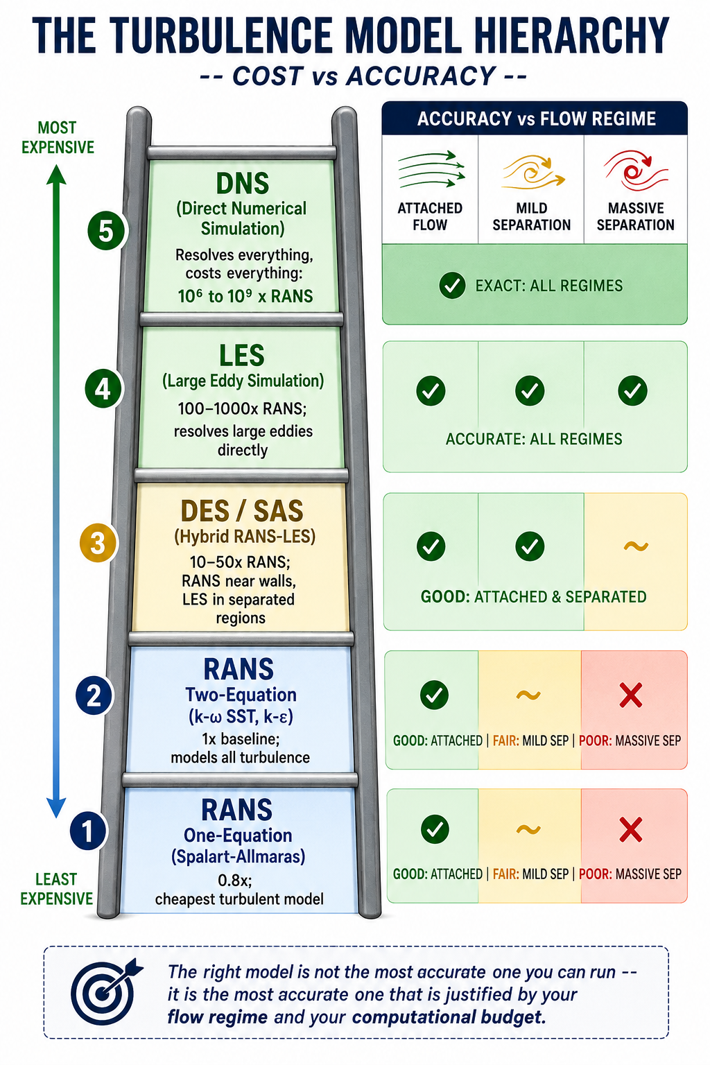
    The turbulence Model Hierarchy

    In a turbine passage, large eddies might span a centimetre. The Kolmogorov scale might be 10 to 50 micrometres. That’s roughly a 1,000-to-1 ratio in length, which becomes a 10⁹ ratio in required computational cells across three dimensions.

    This is why turbulence gets modelled instead of resolved directly. The Navier-Stokes equations describe turbulence exactly, but solving them exactly, called Direct Numerical Simulation (DNS), requires meshes of 10¹² to 10¹⁶ cells and thousands of years of compute time at engineering Reynolds numbers. DNS is reserved for low-Re academic research and model calibration. Every practical engineering simulation needs a modelling strategy.

    Three Strategies for Handling the Eddy Cascade

    Model everything (RANS). Reynolds-Averaged Navier-Stokes models time-average the governing equations, removing turbulent fluctuations and replacing their effect with a turbulent viscosity term. RANS gives a single steady-state flow field. It’s the fastest approach and handles attached or mildly separated flow well.

    Resolve the large eddies, model the small ones (LES and hybrids). Large Eddy Simulation filters the equations to resolve large, energy-containing eddies directly while modelling only the sub-grid scale eddies. It’s far more accurate than RANS for separated flows, but cost scales roughly with Re², making full LES impractical for high-Reynolds-number engineering problems.

    Hybrid RANS-LES. Methods like Detached Eddy Simulation (DES) and Scale-Adaptive Simulation (SAS) use RANS near walls, where it’s accurate and cheap, and switch to LES-like behavior in separated regions, where large unsteady eddies dominate. This captures the physics that matters most at roughly 10 to 50 times RANS cost, versus 100 to 1,000 times for full LES.
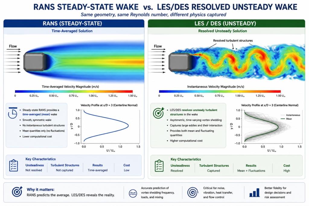
    A split-screen comparison graphic showing a RANS steady-state wake versus an LESDES resolved unsteady wake behind the same bluff body, with labels for time-averaged and resolved turbulent structures.

    RANS Models: The Workhorses of Industrial CFD

    RANS handles the large majority of engineering CFD work, from automotive aerodynamics to HVAC design to turbomachinery. Knowing what each model is calibrated for, and where it breaks down, is the core practical knowledge.

    Spalart-Allmaras: One Equation, One Purpose

    Developed by Spalart and Allmaras at Boeing in 1992, this is the simplest widely used turbulence model. It solves a single transport equation for turbulent kinematic viscosity directly, skipping the k-epsilon or k-omega equations. That makes it the cheapest and most numerically robust RANS option.

    SA was built specifically for external aircraft aerodynamics in attached or mildly separated flow, calibrated on flat plate and aerofoil boundary layers. It remains standard in NASA’s CFD codes. It is not designed for free shear flows, strongly separated flows, or anisotropic turbulence. Using it on a bluff body or a post-stall wing will produce wrong results no matter how good the mesh is.

    The k-epsilon Family: Robust but Flawed Near Walls

    Standard k-epsilon (Jones and Launder, 1972) was the first widely adopted two-equation model and remains common in non-aerospace industrial CFD. Its known weakness is poor near-wall behavior: the epsilon equation goes singular near the wall, forcing reliance on wall functions and limiting its usefulness where near-wall physics matters. In adverse pressure gradients, it over-predicts skin friction and delays predicted separation.

    Realizable k-epsilon (Shih et al., 1994) improves on this by making the C_mu coefficient vary with local strain rate and enforcing mathematical realizability constraints. It performs noticeably better for round jets, mixing layers, and mildly separated flows, making it the preferred choice for combustion chambers and industrial internal flows.

    k-omega SST: Why It Became the Default

    Developed by Florian Menter and published in 1994, k-omega SST is now the standard model for industrial external aerodynamics and the default in most general-purpose solvers. It fixes the two biggest weaknesses of its predecessors: k-epsilon’s poor near-wall behavior and standard k-omega’s oversensitivity to freestream conditions.

    SST does this with a blending function that transitions between k-omega near walls, where it gives excellent near-wall accuracy without wall functions at y+ below 1, and k-epsilon in the freestream, where it’s more robust. The switch is automatic based on wall distance. A built-in stress limiter also prevents over-production of turbulent viscosity in adverse pressure gradients, one reason SST predicts separation onset more accurately than either parent model, as detailed in Menter’s original AIAA paper introducing the model.

    SST isn’t perfect. It still under-predicts separation onset in strongly adverse pressure gradients and misrepresents massively separated flow. A cylinder in crossflow, a stalled wing, or a blunt truck rear will all produce results that mesh refinement cannot fix. Those cases need a higher-fidelity model, or explicit acknowledgment that the RANS result carries large uncertainty.

    Reynolds Stress Model: When Anisotropy Matters

    Two-equation models rely on the Boussinesq assumption, that turbulent stress is proportional to mean strain rate. That assumption breaks down under strong swirl, curvature, buoyancy, or multiple concurrent shear stresses.

    The Reynolds Stress Model solves transport equations for all six Reynolds stress components directly, abandoning Boussinesq. It handles anisotropic turbulence correctly, which helps for rotating machinery, strongly swirling combustors, and buoyancy-driven flows. The cost is 3 to 5 times higher than two-equation models, and it’s numerically less stable. For most industrial work, the accuracy gain over SST doesn’t justify the cost. Reserve RSM for cases where anisotropy is the governing physics, not a minor correction.

    The 10-Model Comparison

    Cost is relative to standard k-epsilon at equivalent mesh density. Accuracy is assessed separately for attached and separated flow, since these are fundamentally different challenges for a turbulence model.

    ModelTypeCost vs RANS k-eAttached Flow AccuracySeparated Flow AccuracyBest Use CaseAvoid When
    Spalart-AllmarasRANS0.8xGood for thin boundary layersPoorThin airfoil, attached aeroAny significant separation
    k-epsilon (standard)RANS1.0xModerate; poor near wallsPoorInternal duct/pipe flowsNear-wall or adverse gradient regions
    k-epsilon (Realizable)RANS1.05xBetter for jetsStill poor for massive separationJet mixing, combustionHigh-AoA aerodynamics
    k-omega (standard)RANS1.0xExcellent near-wallPoor in freestreamNear-wall/transitional flowFreestream-dominated problems
    k-omega SSTRANS1.1xExcellentModerateDefault for most external/internal flowMassively separated/bluff wake flows
    Reynolds Stress ModelRANS3-5xExcellent for anisotropic turbulenceBetter than 2-eqRotating machinery, swirl, buoyancyGeneral use (high cost, marginal gain)
    DESHybrid10-50xGoodGoodHigh AoA, bluff bodies, separated wakesThin boundary layers, unrefined RANS zone
    SASHybrid5-20xGoodGood for massive separationDES alternativeWeakly separated flows
    LESScale-resolving100-1000xExcellentExcellentAeroacoustics, fundamental studiesHigh-Re engineering flows (Re > 10^6)
    DNSExact10^6-10^9xExactExactAcademic turbulence researchAny engineering application

    When RANS Isn’t Enough: DES, SAS, and LES

    If a flow has large-scale, energetic, unsteady separation that governs the quantity you care about (drag, pressure fluctuation, noise, heat transfer in a separated region), RANS gives the wrong answer regardless of which two-equation model you pick. Time-averaging removes exactly the dynamics that dominate these flows.

    Detached Eddy Simulation: The Practical Hybrid

    Introduced by Spalart and colleagues in 1997, DES uses RANS in the attached boundary layer and switches to LES-like treatment in the separated region, based automatically on local mesh size relative to the model’s length scale. The widely used variant, Delayed DES (DDES), adds a shielding function to stop the model from switching to LES prematurely inside thick boundary layers, which early DES implementations sometimes did, causing modelled stress depletion and incorrect wall shear stress.

    DES gives significantly better results than SST for bluff body aerodynamics, aerofoils near stall, and any separated flow where force coefficients or vortex structure matter. The 10 to 50 times cost penalty is real but manageable for problems where RANS produces 20 to 30 percent errors.

    LES: When Only Resolved Unsteady Physics Will Do

    LES is the right choice for aeroacoustics, where noise comes from turbulent pressure fluctuations at frequencies RANS can’t resolve, and for heat transfer in highly unsteady separated regions. Its biggest constraint is the near-wall mesh requirement: at Re = 10⁶, wall-resolved LES needs cell sizes on the order of micrometres, making a full vehicle or aircraft prohibitively expensive. Wall-modelled LES (WMLES), which blends a RANS-like near-wall model with outer-region LES, reduces this cost and is an active area of commercial solver development.

    Scale-Adaptive Simulation: A DES Alternative

    SAS, developed by Menter and Egorov, adds a von Karman length scale term to the omega equation instead of relying on DES’s grid-based trigger. It activates when the local flow length scale drops below the RANS equilibrium scale, letting the model resolve turbulent structures without needing a carefully designed RANS-to-LES transition mesh. In practice, SAS gives similar results to DES for strongly separated flows and is often more robust in transition regions.

    Turbulence Model Selection for 12 Engineering Applications

    This table is a starting reference, not a substitute for project-specific validation.

    Engineering ProblemRecommended ModelWhyWatch For
    Aircraft wing at cruisek-omega SSTBest near-wall accuracy for attached flowMay predict separation 2-3° too late at high AoA
    Automotive exterior (sedan)SST for baseline; DES for wake detailSST gives Cd within 5-8%; DES resolves unsteady wakeSST can under-predict blunt-rear separation by 10-20%
    Circular cylinder in crossflowDES or LESRANS misrepresents wake width and shedding frequencyRun at least 10 shedding periods before extracting statistics
    Internal pipe flow (developed)k-omega SST or Realizable k-epsilonWell-captured by either two-equation modelConfirm y+ matches chosen near-wall treatment
    HVAC room airflowSST with Boussinesq buoyancyStandard for room CFD; buoyancy term essentialDiffuser modelling detail strongly affects jet throw
    Wind around a tall buildingSST with ABL modifications; LES for pedestrian comfortHandles time-averaged wind loadsInlet profile must match ABL log-law and roughness
    Gas turbine blade coolingSST with gamma-Re_theta transitionCaptures laminar-to-turbulent onset for heat transferRequires accurate inlet turbulence intensity
    Centrifugal pump impellerSST in rotating frame (MRF or sliding mesh)Handles body forces and secondary flowsNeeds rotation-corrected turbulence production term
    Combustion chamber / burnerRealizable k-epsilon or RSM with combustion modelCompatible with combustion models; RSM better for swirlInclude radiation model for high-temperature flames
    Aeroacoustic noise from aerofoilLES with Ffowcs Williams-Hawkings analogyOnly LES resolves noise-generating structuresMesh must resolve eddies at frequencies of interest
    Ship hull resistanceSST with Volume of Fluid (VOF)Standard for hydrodynamics; VOF captures wave resistanceFree surface mesh needs 20+ cells per wave height
    Blood flow through a stentLaminar/transitional SST with Carreau non-Newtonian modelPhysiological Re is mostly laminar to transitionalRequires pulsatile BCs from measured waveforms

    Understanding Model Constants

    Every turbulence model contains empirical constants calibrated against experimental data for specific canonical flows. These aren’t free parameters to tune for a better match on one result. Adjusting them to fit a specific experiment is curve-fitting, not physics, and the modified constants will produce wrong results for any flow outside the case they were tuned to.

    ModelKey ConstantDefaultControlsWhen to Modify
    k-omega SSTa1 (stress limiter)0.31Max ratio of shear stress to kRarely; some codes use 0.302
    k-omega SSTbeta* (k dissipation)0.09Dissipation-to-k-omega relationshipNever
    k-epsilon standardC_mu0.09Overall turbulence levelSometimes 0.06-0.07 for round jets
    k-epsilon standardC1_epsilon, C2_epsilon1.44, 1.92Production/destruction in epsilon equationOnly with specific swirl validation
    Spalart-Allmarascb1, cb2, cv10.1355, 0.622, 7.1Production, destruction, viscosity ratioOnly for transition modeling

    The only legitimate reasons to change a constant: a published, peer-reviewed modification exists for a known model deficiency in your specific flow class, or you’re calibrating a transition model against measured data for one specific geometry and condition. Any other adjustment turns the simulation into result-tuning with zero predictive value for new conditions, even if it matches the calibration case perfectly.

    Laminar-to-Turbulent Transition

    Standard RANS models assume fully turbulent flow from the inlet. That’s fine at high Reynolds numbers, but for gas turbine blades at altitude, fan and compressor blades, low-speed wind turbine aerofoils, and small propellers, a meaningful part of the surface may still be laminar. Treating it as turbulent overestimates skin friction and misrepresents heat transfer.

    The gamma-Re_theta transition model, developed by Menter, Langtry, and colleagues as an add-on to SST, solves two extra transport equations: one for intermittency (the fraction of time flow is turbulent at a point) and one for the transition momentum thickness Reynolds number. It compares local flow conditions against empirical transition-onset correlations and progressively activates the full turbulence model across the transition region.

    This model matters most for gas turbine blade heat transfer, where laminar-versus-turbulent regions shift the local Nusselt number by a factor of 3 to 5, and for low-speed aerofoil performance, where leading-edge laminar separation bubbles govern maximum lift. It adds roughly 20 percent compute cost and needs correct freestream turbulence intensity to predict bypass transition accurately.

    Practical Setup: Getting the Inlet Values Right

    For k-omega SST, turbulent kinetic energy k and specific dissipation rate omega must be set at every inlet. Getting them wrong rarely causes divergence, but it shifts turbulence levels throughout the domain, especially near separated regions.

    GIVEN: Freestream velocity V, turbulence intensity Tu, length scale L
    
    k = 1.5 * (V * Tu)^2
    Example: V=50 m/s, Tu=0.005 -> k = 1.5 * (0.25)^2 = 0.9375 m^2/s^2
    
    omega = k^0.5 / (C_mu^0.25 * L), where C_mu = 0.09
    Example: k=0.9375, L=0.01m -> omega ≈ 176.6 s^-1
    
    epsilon = C_mu^0.75 * k^1.5 / L (for k-epsilon)
    Example: k=0.9375, L=0.01m -> epsilon ≈ 14.9 m^2/s^3
    
    Turbulent viscosity ratio target: 1-10 for low-Tu freestream; 10-100 for internal flows
    

    Turbulence intensity guide:

    • Low-turbulence wind tunnel: 0.05 to 0.3 percent
    • Atmospheric boundary layer: 5 to 15 percent
    • Industrial pipe/duct flow: 3 to 8 percent
    • Turbomachinery inlet: 3 to 10 percent
    • Combustion chamber inlet: 5 to 20 percent

    Turbulent length scale guide:

    • Pipe/duct flow: 0.07 × hydraulic diameter
    • Flat plate: 0.4 × boundary layer thickness
    • Wind tunnel: 0.01 × tunnel width
    • Atmospheric: 100 to 300 m at reference height

    Steady RANS vs. URANS

    URANS is appropriate when large-scale unsteadiness is periodic and much larger in scale than turbulence itself: vortex shedding, periodic stall, pulsatile pipe flow. It’s not a substitute for LES. It still models all turbulence, but lets large-scale unsteady structure develop instead of being averaged away.

    If a steady RANS run oscillates and won’t converge, that’s a signal the flow is unsteady, not a convergence problem to push through with more iterations. Either time-average a URANS result or move to DES or LES. An arbitrary instantaneous snapshot of an unsteady solution has no defined physical meaning.

    Running a Turbulence Model Sensitivity Study

    For any result feeding a design decision, run the same geometry, mesh, and boundary conditions through two or three models (say, SST, Realizable k-epsilon, and Spalart-Allmaras for external aero) and compare. Agreement within 5 percent for Cd and 2 percent for Cl means turbulence model choice isn’t the dominant uncertainty. Disagreement above 10 percent means it is, and the choice needs justification against experimental or higher-fidelity data.

    A Cp comparison along the surface also shows where the models diverge: leading edge points to transition or stagnation issues, suction surface points to adverse pressure gradient handling, trailing edge points to separation and base pressure.

    Worked Examples

    Wind load on a low-rise industrial building: A team needed pressure coefficients on a 10m tall, 40m wide, 20m deep building in open terrain for structural loading. They used k-omega SST with an ABL inlet profile matched to a roughness length of 0.03m, generating 15 percent turbulence intensity at roof height. Time-averaged Cp on windward and side walls landed within 10 to 15 percent of wind tunnel data, adequate for code compliance.

    The roof was the exception: leading-edge separation over the first 20 to 30 percent of the roof width under-predicted suction by 15 to 25 percent, since SST can’t fully capture that separated zone. LES or wind tunnel data would be needed if the roof were the governing structural case.

    Pump impeller at part-load: At 60 percent of design flow, incidence angle at the impeller inlet risked leading-edge separation and rotating stall. The team used SST in a rotating reference frame with sliding mesh for full transient impeller-volute interaction, since steady MRF averages away the tongue-blade interaction that dominates at off-design. Running through 5 impeller revolutions after reaching a stationary state gave head and efficiency predictions within 3 to 5 percent and 2 to 3 percentage points of the test curve at design point, with correct off-design trends even where absolute values differed by 5 to 10 percent.

    Frequently Asked Questions

    What is the best turbulence model for CFD? There isn’t one. k-omega SST is the industry standard for attached or mildly separated external aerodynamics. Massively separated flows need DES or LES. Aeroacoustics requires LES, since RANS can’t predict the pressure fluctuations that generate noise. Start with SST, validate against a reference, and upgrade only when SST shows a real discrepancy in the regime that matters.

    What’s the difference between k-omega and k-omega SST? Standard k-omega has excellent near-wall behavior but is highly sensitive to the omega value set at the freestream inlet, which makes it unreliable for external flows. SST blends k-omega near walls with k-epsilon in the freestream, switching automatically based on wall distance, and adds a stress limiter that improves separation prediction. That combination is why SST outperforms both parent models for external aerodynamics.

    When should I use DES instead of RANS? When the flow is separated over a significant area at your operating condition, and the drag, pressure distribution, or acoustic output you’re predicting depends on the structure of that separated region. Common triggers: bluff bodies with large wakes, aerofoils within 3 to 5 degrees of stall, deployed flaps or spoilers, and any case where unsteady loads or vortex structure matter. Budget 10 to 50 times the cost of SST.

    Can I use RANS for unsteady problems? Yes, as URANS, when the dominant unsteadiness is large-scale and periodic, like vortex shedding or pulsatile flow. It’s not appropriate when the unsteadiness comes from the turbulence itself or from separated-region dynamics at a scale close to the turbulence scale; those cases need DES or LES.

    How much does turbulence model choice affect the final result? For attached flow, different RANS models typically agree within 3 to 8 percent for drag and 1 to 3 percent for lift, so model choice isn’t the dominant error source. For separated flows, RANS models can disagree by 20 to 50 percent, making model choice the largest source of uncertainty. For acoustics, RANS is wrong by orders of magnitude regardless of model, since it averages away the noise source entirely.

    What does y+ have to do with turbulence model selection? Different models need the first wall cell in different parts of the boundary layer. Low-Re models and SA need y+ below 1. Standard wall functions need y+ between 30 and 300. Mismatching the mesh to the model, or landing in the 5-to-30 buffer layer, produces wall shear stress errors of 10 to 40 percent regardless of which model you chose. Decide the near-wall treatment before generating the mesh, then check y+ post-solution.

    Key Takeaways

    Turbulence model selection isn’t about running the most accurate model available. It’s about matching the physics that governs your quantity of interest to a cost justified by the engineering decision at hand. LES on a duct pressure drop wastes compute resolving detail that changes the answer by under 1 percent. SST on a bluff body aeroacoustics problem gives noise predictions wrong by orders of magnitude. Both are the wrong choice, just in opposite directions.

    Start by classifying the flow: attached, mildly separated, or massively separated. Attached flow needs SST or SA. Massive separation needs DES or LES. Mild separation needs SST plus a sensitivity study against a higher-fidelity reference. Then check secondary physics: rotation needs correction terms, transition needs the gamma model, strong anisotropy may need RSM. Finally, match the near-wall treatment and mesh to the y+ range that treatment requires.

    None of this removes the need for validation against a reference before trusting a result for a design decision. The models here have documented accuracy ranges and known failure modes. Working inside those ranges, with validation, gives reliable results. Working outside them without validation gives results indistinguishable from wrong ones.
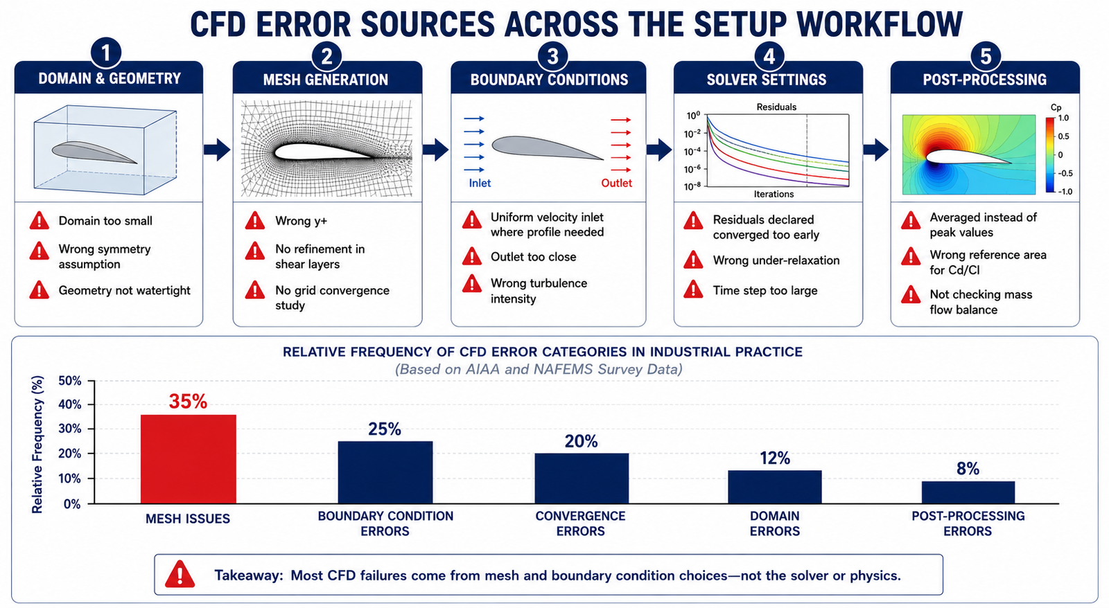
  • Common CFD Setup Mistakes and How to Avoid Them (20-Point Guide)

    Common CFD Setup Mistakes and How to Avoid Them (20-Point Guide)

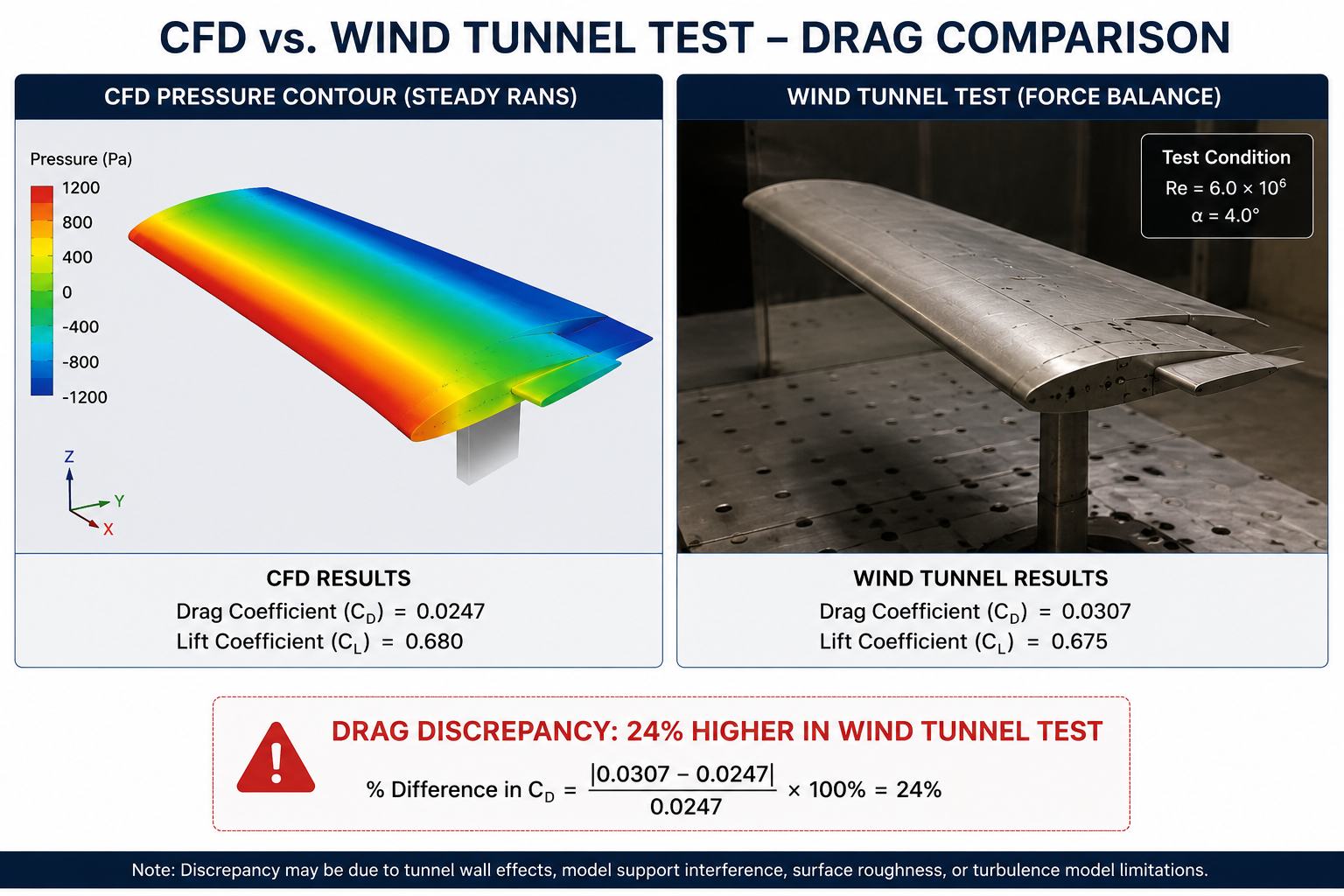
    A recent CFD run took four days to set up and 16 hours to run on a 128-core cluster. The predicted drag coefficient was 0.287. The wind tunnel measurement for the same configuration was 0.231. That’s a 24 percent error, and it had nothing to do with turbulence model uncertainty or geometry mismatches.

    The real cause was three stacked setup errors: a domain that ended too soon behind the wing, a first-cell y+ value stuck in the unreliable buffer layer, and a convergence call made from residuals alone while the drag coefficient was still drifting. Each error alone would have cost 5 to 10 percent accuracy. Together, they made the result useless for the design decision it was meant to support.

    Quick answer: The most common CFD setup mistakes fall into five categories: domain and geometry, mesh quality, boundary conditions, solver settings and convergence, and post-processing. None of them show up as solver errors. The simulation still converges, the plots still look smooth, and the numbers still look plausible. That’s what makes them dangerous, and why systematic checking, not visual inspection, is the only reliable way to catch them.

    CFD drag prediction versus wind tunnel measurement showing 24 percent discrepancy caused by CFD  setup mistakes errors

    CFD setup mistakes happen before the solver ever runs, in decisions about domain size, mesh topology, boundary conditions, and solver parameters. Like FEA preprocessing errors, they produce output that looks completely valid: smooth contours, stable force coefficients, clean convergence histories. The solver never flags them. Only systematic verification, domain independence, mesh independence, y+ checks, mass conservation, and monitored-quantity convergence, can catch them before a bad result reaches a design review.

    The 20 Most Common CFD Setup Mistakes at a Glance

    The table below lists all 20 mistakes by category, typical error magnitude, how to detect them, and priority. Critical items produce errors above 10 percent and cannot be trusted without correction. High priority items introduce meaningful risk that compounds with other errors. Medium items are good practice that improves reliability and prevents downstream post-processing problems.

    #MistakeCategoryTypical ErrorDetection MethodPriority
    1Domain too smallDomain / Geometry5–30% in force coefficientsExtend boundaries and rerun; compare resultsCritical
    2Wrong turbulence model for the regimePhysics10–50% drag error in separated flowCompare RANS vs DES/LES against test dataCritical
    3y+ wrong for the near-wall modelMesh10–40% skin friction errorCheck y+ distribution post-solveCritical
    4Insufficient mesh in shear layers/wakesMesh10–40% wake drag errorGrid convergence studyCritical
    5Wrong inlet turbulence intensity/length scaleBoundary Conditions5–20% error in transition/separationMatch Tu and length scale to real conditionsHigh
    6Outlet too close to the bodyBoundary ConditionsDivergence or false backflowMove outlet 10–20 diameters downstreamCritical
    7Symmetry plane on asymmetric flowBoundary ConditionsFundamentally wrong resultVerify symmetry with a full-domain reference runCritical
    8Wrong pressure-velocity coupling schemeSolver SettingsSlow convergence or divergenceUse COUPLED for high-Re external aeroHigh
    9Convergence declared from residuals aloneConvergence5–25% errorMonitor lift, drag, and mass flow vs. iterationCritical
    10Too few iterations for steady stateConvergenceScattered, unstable averagesRun until monitors vary < 0.1% over 200 iterationsHigh
    11Wrong reference area/velocity for Cd/ClPost-processingError equal to the ratio of areas usedDocument reference values before computingHigh
    12Averaged instead of peak values reportedPost-processing10–40% under-reporting at peaksUse unaveraged, cell-centred values at critical pointsHigh
    13Wall functions applied at y+ < 30Mesh10–30% skin friction over-predictionTarget 30 < y+ < 300 for wall functionsHigh
    14Missing refinement at leading/trailing edgesMeshWrong pressure distribution, circulationCluster mesh at stagnation and wake regionsHigh
    15Periodic BC on non-periodic flowBoundary ConditionsArtificial forced periodicityVerify true periodicity before applyingMedium
    16Wrong fluid properties at operating temperaturePhysicsRe error scales all downstream resultsCompute Re from actual target conditionsHigh
    17Time step too large in transient runsSolver SettingsAliased or missed unsteady featuresKeep Courant number in the recommended rangeHigh
    18Mass flow imbalance not checkedConvergenceNon-physical pressure and force fieldsConfirm imbalance < 0.1% of inlet mass flowCritical
    19Default under-relaxation for all casesSolver SettingsDivergence or oscillationReduce to 0.3–0.5 for difficult problemsMedium
    20No grid convergence studyMeshUnknown discretisation errorRun coarse/medium/fine mesh; report GCICritical

    Category 1: Domain Size and Geometry

    Domain size errors are the hardest CFD mistakes to catch from a single run. A domain that’s too small still converges cleanly and looks physically reasonable. The error only surfaces when you enlarge the domain and the results shift, or when you compare against test data and find a systematic bias.

    Mistake 1: Domain Too Small

    The downstream extent is the dimension analysts underestimate most. If the outlet boundary intersects the wake, or the body’s pressure field reaches it, the outlet condition distorts pressure around the body and skews the drag prediction. Lateral extents should keep blockage ratio below roughly 5 percent.

    How to check it: run the original domain, then extend every boundary by 50 percent and rerun. If drag or lift changes by more than 1 percent, the domain was too small. This domain independence study should be standard practice before any result is reported.

    Flow ConfigurationInlet DistanceOutlet DistanceLateral ExtentTop/Bottom Extent
    External aerofoil/wing (2D)10–15 chords20–30 chords10–15 chords10–15 chords
    External body (car, building), 3D5–10 lengths15–20 lengths5 widths each side5 heights + ground clearance
    Internal duct/pipe flow10–20 diameters30–50 diametersWall boundaryWall boundary
    Bluff body (cylinder, facade)10 diameters30–40 diameters10 diameters each side10 diameters
    Turbomachinery blade passage1–2 chords2–3 chordsPeriodic at blade pitchPeriodic or hub/tip wall
    Wind over terrain (ABL)5–10 building heights15–20 building heights5 heights each side6 heights or to gradient height

    Mistake 7: Symmetry Applied to Asymmetric Flow

    A symmetry plane halves the computational cost, but only when the physics is genuinely symmetric. Many flows that look symmetric aren’t. A cylinder produces an alternating vortex street. A sphere develops an off-axis wake at moderate Reynolds number. A wing at high angle of attack can separate asymmetrically even with symmetric geometry.

    Forcing symmetry on an asymmetric flow produces wrong separation onset, wrong stall angle, and often solver oscillation as it fights the imposed constraint. Test it with a full-domain run and no symmetry plane. If the result is symmetric to within 0.1 percent, the assumption holds.

    Category 2: Mesh Quality and Refinement

    Mesh errors cause roughly 35 percent of all CFD accuracy problems in industrial practice, making this the single largest error source. Unlike domain errors, mesh errors can be local, affecting only a poorly resolved feature, which makes them harder to catch with a simple sensitivity study.

    Mistake 3: Wrong y+ Value for the Near-Wall Treatment

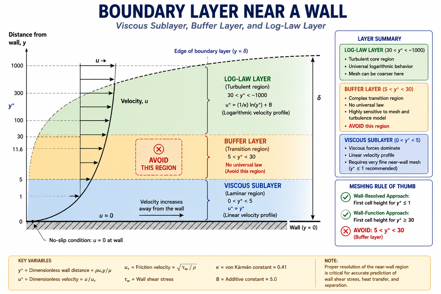
    The y+ value of the first wall cell determines which part of the boundary layer that cell sits in. Below 5 is the viscous sublayer. Between 5 and 30 is the buffer layer, where neither wall functions nor low-Re models are accurate. Above 30 is the log-law layer.

    Wall functions are only valid in the log-law region, typically y+ between 30 and 300. Landing in the buffer layer produces wall shear stress errors of 10 to 40 percent. Low-Reynolds-number models resolve the sublayer directly but need much finer meshes, usually 15 to 20 cells across the boundary layer with the first cell at y+ below 1.

    Near-Wall Treatmenty+ TargetWhat Happens if WrongWhen to Use
    Low-Re (resolves boundary layer)y+ < 11–5: transition error; > 5: wall function takes overSkin friction drag, heat transfer, turbine cooling
    Standard wall functions30 < y+ < 300< 30: over-predicts shear; > 300: too coarseAttached turbulent boundary layers, cruise aero
    Enhanced wall treatmentAny, avoid 5–30Buffer layer wrong for both modelsGeneral use when y+ is uncertain
    Scalable wall functionsy+ ≥ 11.25 (enforced)Less accurate than low-Re, but avoids divergenceCoarse meshes, ±10–15% accuracy acceptable
    Boundary layer diagram showing y+ zones including the buffer layer to avoid in CFD near-wall meshing

    Mistake 20: No Grid Convergence Study

    Reporting a single-mesh result as your final answer isn’t defensible engineering practice. Every CFD solution carries discretisation error, the gap between the numerical result on a finite mesh and the true solution on an infinitely fine one. That error can range from 0.1 to 30 percent depending on flow complexity and mesh quality.

    The standard method for quantifying it is the Grid Convergence Index (GCI), defined by Celik et al. in the ASME Journal of Fluids Engineering. The procedure: run three systematically refined meshes, compute the observed order of convergence, then calculate GCI as a percentage uncertainty band on the fine-mesh result. Below 3 percent is acceptable for most engineering work. Below 1 percent is the bar for certification-grade results.

    Worked example:

    Coarse mesh (500,000 cells):   Cd = 0.312
    Medium mesh (2,000,000 cells): Cd = 0.295
    Fine mesh (8,000,000 cells):   Cd = 0.289
    
    Refinement ratio r = 4^(1/3) = 1.587
    Observed order p = ln(|-0.017 / -0.006|) / ln(1.587) ≈ 2.25
    Richardson extrapolated Cd ≈ 0.286
    GCI (fine mesh) ≈ 1.4%
    
    Result: Cd = 0.289 ± 1.4% (acceptable for engineering; < 3% target)
    

    Category 3: Boundary Condition Errors

    CFD boundary conditions prescribe the flow state, velocity, pressure, temperature, turbulence, at every domain boundary. The solver builds the interior solution from those values. Get the boundary wrong, and the interior solution is wrong even if the mesh and turbulence model are perfect.

    Inlet BC TypeWhen CorrectCommon Mistake
    Velocity inlet (uniform)Known uniform freestreamApplied to non-uniform duct flow
    Velocity inlet (profile)Complex upstream history mattersSkipped when profile data is available
    Pressure inletPressure-driven flow (fans, buoyancy)Used when mass flow is actually known
    Mass flow inletMetered or fixed-delivery systemsUsed at compressible high-speed inlets
    Periodic/cyclicTruly repeating geometry and flowApplied without verifying periodicity
    Turbulence intensity + length scaleAlways requiredLeft at solver default (5%)

    Mistake 5: Wrong Inlet Turbulence Intensity

    This is one of the most frequently mis-set boundary parameters, largely because analysts leave it at the solver default of 5 percent instead of matching it to the real upstream source.

    • Low-turbulence wind tunnel: 0.05 to 0.3 percent
    • Atmospheric boundary layer: 5 to 20 percent, matched to a log-law profile
    • Industrial fan or blower discharge: 3 to 8 percent
    • Fully developed pipe flow: roughly 2 to 5 percent

    Using the 5 percent default in a low-turbulence wind tunnel case inflates inlet turbulence energy by a factor of 15 to 100, artificially delaying separation and skewing the stall prediction.

    Mistake 6: Outlet Boundary Too Close to the Body

    A pressure outlet only behaves correctly when the flow there is roughly parallel with small velocity gradients, conditions that exist well downstream of any wake or recirculation. If the outlet sits too close, the prescribed pressure propagates upstream and distorts the flow around the body.

    The tell-tale sign: isobars near the outlet curve toward the boundary instead of running parallel to it. If the wake velocity deficit at the outlet exceeds 5 percent of freestream, move the outlet back. For highly separated flows, that can mean 30 to 50 body diameters downstream, further than most analysts initially expect.

    Category 4: Solver Settings and Convergence

    These are the most deceptive mistakes because they leave no visible trace in the output. A run with wrong under-relaxation, wrong convergence criteria, or too large a time step looks identical to a correctly configured one.

    Mistake 9: Declaring Convergence From Residuals Alone

    Residuals measure the global imbalance of the governing equations across every cell. Standard guidance says to run until residuals drop 3 to 4 orders of magnitude. That’s necessary, but not sufficient.

    A simulation can show residuals down 6 orders of magnitude while drag is still changing by several percent every 100 iterations. This happens because a small, slowly evolving region, a separation bubble or corner vortex, can be invisible to the global residual while still driving the forces you actually care about. Monitor lift, drag, and mass flow directly. Declare convergence when those stabilize, not when residuals hit a target.

    Convergence IndicatorAdequate ValueRecommended Action if Not Met
    Residual (continuity)< 1×10⁻⁴ engineering; < 1×10⁻⁶ high-accuracyContinue iterating; check mesh quality
    Residual (momentum)< 1×10⁻⁴ engineering; < 1×10⁻⁵ aeroCheck mesh; reduce time step for transient
    Cd stabilisation< 0.1% change over last 200 iterationsContinue iterating; consider transient RANS
    Cl stabilisation< 0.1% change over last 200 iterationsTime-average or switch to unsteady
    Mass flow imbalance< 0.1% of inlet mass flowCheck for boundary or geometry errors

    Mistake 18: Not Checking Mass Flow Imbalance

    Mass conservation is the most basic requirement of any incompressible CFD solution. Inlet mass flow should equal outlet mass flow to within 0.1 percent. A larger imbalance means the run hasn’t converged, or there’s a geometry gap or boundary condition mismatch letting mass leak through a wall.

    This is the simplest, most reliable check available and should be the first thing you look at, before force, pressure, or temperature results. If mass isn’t conserved, nothing downstream is trustworthy.

    Category 5: Post-Processing Errors

    These mistakes happen after a correctly run simulation, in how the results get extracted, displayed, or interpreted. They’re the CFD equivalent of FEA post-processing errors.

    Mistake 11: Wrong Reference Values for Force Coefficients

    Cd = Drag / (0.5 × ρ × V² × A_ref). The reference area A_ref isn’t universal:

    • Aircraft: wing planform area
    • Automobiles: frontal projected area
    • Bluff bodies: frontal projected area (diameter × length, or πd²/4 for a sphere)
    • Buildings: depends on loading direction

    Using the wrong reference area shifts Cd by the ratio between the correct and incorrect areas, which can be 20 to 50 percent for geometries where planform and frontal area diverge significantly. Document the reference area used before publishing any coefficient, and confirm it matches when comparing across codes or against test data.

    Mistake 12: Averaged Instead of Peak Values

    Contour plots often average nodal values from surrounding elements. At high-gradient locations, stagnation points, suction peaks, separation onset, that averaging can under-report the true peak by 10 to 40 percent. For surface Cp plots, always pull unaveraged, cell-centred values at critical points. The leading-edge suction peak, in particular, determines boundary layer transition and is exactly where averaging does the most damage.

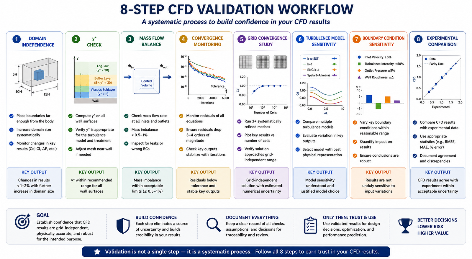
    Eight-step CFD validation workflow from domain independence check to experimental comparison

    The CFD Validation Workflow

    No single check catches every mistake. Domain independence doesn’t catch y+ errors. y+ checks don’t catch convergence errors. The full workflow runs every check in sequence:

    1. Domain independence: extend each boundary 50 percent and compare Cd, Cl, and surface Cp. Repeat until results change less than 1 percent.
    2. y+ check: plot y+ on all walls after the first converged run and confirm it matches your near-wall model.
    3. Mass flow balance: confirm imbalance is under 0.1 percent of inlet mass flow.
    4. Convergence by monitored quantities: track Cd, Cl, mass flow, and pressure versus iteration, not just residuals.
    5. Grid convergence study: run coarse, medium, and fine meshes and report GCI.
    6. Turbulence model sensitivity: compare two models (for example, SST versus Realizable k-ε). Agreement within 5 percent means model choice isn’t the dominant uncertainty.
    7. Boundary condition sensitivity: vary uncertain inlet turbulence by a factor of 3 and check the impact.
    8. Comparison with reference data: validate against a known analytical or experimental case before trusting the target geometry result.

    What a Reportable CFD Result Must Include

    A CFD result isn’t ready for an engineering decision unless it documents: domain extent and independence study, mesh count and y+ distribution with GCI, turbulence model and justification, boundary conditions with values, convergence history of monitored quantities, mass flow balance, and reference values for any force coefficients. Without this, the result can’t be peer-reviewed, reproduced, or trusted.

    Worked Examples

    Domain independence failure, ground vehicle aerodynamics: A team ran a 3D RANS simulation at highway speed with an 8-vehicle-length downstream domain and got Cd = 0.298. Extending to 20 lengths dropped Cd to 0.271, a 9.1 percent change. The outlet had been sitting inside the vehicle’s near-wake, pulling base pressure down and inflating drag. Had the original number been used for a compliance check against a 0.28 target, the vehicle would have failed a target it actually met.

    False convergence, aerofoil near stall: A NACA 0015 simulation at 15 degrees angle of attack showed residuals down 4 orders of magnitude after 2,000 iterations, reporting Cl = 1.34. Reviewing the Cl history revealed oscillation between 1.28 and 1.41 with a 150-iteration period, meaning it had never actually converged. Switching to unsteady RANS and time-averaging over five shedding periods gave Cl = 1.31 and Cd = 0.094, 8 percent higher than the false-converged steady value.

    Frequently Asked Questions

    How do I know if my CFD domain is large enough? Run a domain independence study. Extend every boundary by at least 50 percent and compare drag, lift, and surface pressure. If any coefficient shifts more than 1 percent, the domain was too small. For external aerodynamics, the downstream boundary is usually the critical one: 15 to 20 body lengths for streamlined shapes, 30 to 50 for bluff bodies.

    What y+ value should I target? Use y+ = 0.5 to 1.0 for low-Reynolds-number models, or 30 to 100 for standard wall functions. Avoid the 5 to 30 buffer layer regardless of which near-wall treatment you’re using.

    Why are my residuals converged but my drag coefficient is still changing? Residuals measure global imbalance, not local flow features. A slowly evolving separation bubble or corner vortex can keep drifting the drag coefficient while contributing almost nothing to the global residual. Monitor drag and lift directly and declare convergence only when they stabilize.

    What is the Grid Convergence Index and do I need to compute it? GCI quantifies the discretisation error in your result, how far the numerical answer sits from the theoretical infinite-mesh solution. For anything feeding a design decision, regulatory submission, or published comparison, yes, you need it. A three-mesh study costs roughly three times a single run but gives you a defensible uncertainty bound.

    How do I handle backflow at my pressure outlet? Move the outlet farther downstream past the recirculation zone; this is the most reliable fix. If that’s not practical, use a backflow prevention option to prescribe flow direction at the boundary, though this only reduces the boundary effect rather than eliminating the underlying accuracy problem.

    What turbulence model should I use? k-ω SST is the standard general-purpose choice for external aerodynamics. For strongly separated flows, switch to DES or LES at significantly higher computational cost. Avoid standard k-ε for external aero; it has worse near-wall behavior than SST with no real advantage.

    Key Takeaways

    CFD setup mistakes happen before the solver runs and produce output that looks completely valid. The 20 mistakes covered here, from an undersized domain through false convergence, account for most CFD accuracy failures in industrial practice. Each has a clear detection method and a known fix.

    Build the verification workflow into your process from the first run, not as damage control after someone questions the result. Domain independence and y+ checks cost one or two extra runs. A GCI study costs about three times a single run. Convergence monitoring costs nothing beyond plotting force coefficients alongside residuals. That’s a small price for results with a documented, defensible uncertainty bound.

  • How CFD Improves HVAC System Performance (With Worked Examples)

    How CFD Improves HVAC System Performance (With Worked Examples)

    The 15,000 m² office building was designed to meet ASHRAE 55 thermal comfort standards. Mechanical calculations confirmed adequate supply airflow, diffuser throw distances, and a 12 air-change rate in every zone, while BMS commissioning data showed that the fans were delivering the required airflow. Yet six months after occupancy, 34% of occupants rated their thermal comfort as unacceptable. The calculations were correct, but the airflow distribution was not. Two of the eight ceiling diffusers created a Coanda jet that travelled directly toward the return grille, short-circuiting about 12% of the supply air before it reached the occupied zone. A far corner received almost no fresh supply air, resulting in elevated CO₂ levels and uncomfortable conditions.

    This illustrates a fundamental HVAC design challenge: correct airflow quantity does not guarantee correct airflow distribution. Manual calculations can determine supply volume, cooling load, and diffuser velocity, but they cannot fully predict how air moves through a complex three-dimensional space. Computational fluid dynamics (CFD) can reveal airflow patterns, temperature distribution, draught risk, short-circuiting, and stagnant zones before commissioning. This article explores the key applications of CFD in HVAC performance, including thermal comfort, duct pressure losses, airflow distribution, cleanrooms, data centres, smoke control, and energy optimization, with practical examples showing how CFD results translate into specific design improvements.

    Where CFD Adds Value in HVAC: The Ten Application Areas

    CFD is not the right tool for every HVAC engineering task. Sizing a duct run, selecting a chiller, or calculating a heating load are manual calculation tasks where CFD adds no value, the physics is one-dimensional and the established methods are accurate. CFD becomes valuable when the flow is three-dimensional and the interactions between geometry, thermal loads, and airflow patterns determine the outcome. The following table maps the ten HVAC application areas where CFD provides information that manual methods cannot, with the physics, key outputs, design decisions enabled, and fidelity level required.

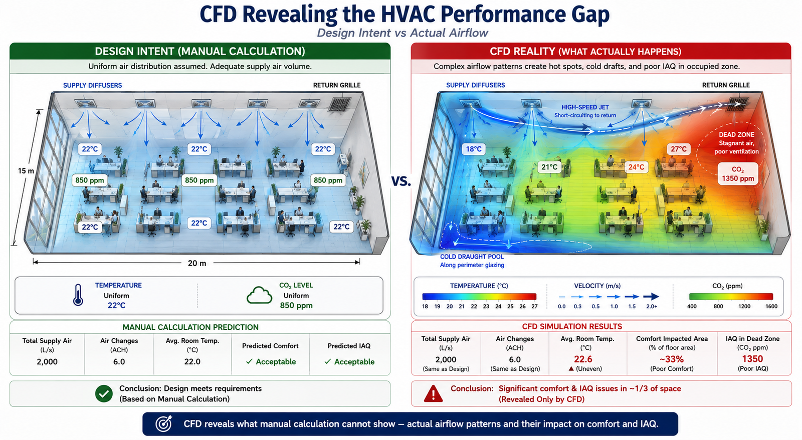
    CFD Revealing the HVAC Performance Gap, Design Intent vs Actual Airflow A split-room diagram showing two side-by-side views of the same open-plan office floor plate (20m × 15m). Left panel labeled 'Design Intent (Manual Calculation)': uniform colour wash across the occupied zone with arrows from ceiling diffusers reaching evenly to all areas; temperature labelled uniformly at 22°C; CO2 labelled uniformly at 850 ppm. Right panel labeled 'CFD Reality': colour temperature contour from cold blue (18°C) near the supply diffusers to warm red (27°C) in the back corner; velocity arrows showing a high-speed jet across the ceiling short-circuiting to the return grille; a dead zone (stagnant red region) in the far corner with CO2 at 1350 ppm; a cold draught pool at floor level near the perimeter glazing. The contrast between left and right panel directly illustrates the core value proposition: CFD reveals what manual calculation cannot show, that the actual airflow pattern delivers poor comfort in a third of the space despite adequate total supply air volume.
    HVAC ApplicationCFD Physics RequiredKey Output MetricsDesign Decision EnabledFidelity Level
    Room airflow distribution and comfort3D RANS with buoyancy; energy equation for temperature; humidity transport optionalAir temperature at 0.6m, 1.1m, 1.7m above floor; air velocity at occupied zone; draught rate (DR) per ISO 7730Diffuser type, location, and throw distance; return grille placement; supply air volume and temperatureMedium, standard RANS k-ω SST; steady-state
    Duct system pressure drop and flow balancing3D RANS in duct network; or 1D network model with CFD-derived loss coefficientsPressure drop per duct section; flow velocity distribution; balancing damper requirementsDuct sizing, transition geometry, elbow radius, junction design; fan selection and speedLow to medium, duct segments can be modeled individually; full-network 1D is most efficient
    Diffuser and grille performance3D RANS with fine mesh at diffuser slots; jet throw predictionJet throw distance; entrainment ratio; Coanda effect along ceiling; terminal velocity at 0.25 m/sDiffuser type selection (linear, radial, displacement); supply angle; slot velocityMedium-High, fine mesh required for slot geometry; validates manufacturer performance curves
    Chilled beam and radiant cooling3D coupled radiation + convection CFD; buoyancy-driven flowMean radiant temperature (MRT); operative temperature; natural convection plume from occupantsChilled beam spacing; supply water temperature; ceiling height requirementsHigh, radiation model required; occupant thermal plume modelling adds complexity
    Clean room and ISO class compliance3D LES or high-quality RANS; particle transport; filtration efficiencyAir change rate; non-uniformity of velocity; particle concentration; pressure differential to adjacent zonesHEPA/ULPA filter placement; number of air changes per hour; supply/return pattern for ISO 14644 complianceHigh, particle tracking and contaminant transport require validated CFD
    Data centre hot aisle/cold aisle cooling3D RANS with server rack power dissipation as volumetric heat source; bypass airflowServer inlet temperature; rack temperature non-uniformity; bypass ratio (cold air short-circuit); PUE impactRack layout; containment design; CRAC unit placement; floor tile perforation patternMedium, simplified rack models acceptable; detailed model for hot aisle containment validation
    Kitchen and laboratory exhaust hood capture3D transient or steady RANS; contaminant species transport; thermal buoyancy from cooking sourceCapture velocity at hood face; contaminant containment at design flow; spillage under cross-draughtHood face velocity; exhaust volume flow; makeup air location to avoid cross-draught interferenceMedium-High, transient better for intermittent loads; species transport adds cost
    Hospital operating theatre ventilation3D RANS; particle transport; unidirectional flow (UDF) validationSurgical site air cleanliness; particle counts in critical zone; ISO 14644 zone boundaryUDF canopy dimensions; supply velocity; supply air temperature; recirculation avoidanceHigh, regulatory compliance requires detailed particle transport validation
    Natural ventilation / mixed-mode buildings3D CFD with wind boundary conditions + buoyancy; external + internal domains coupledAir change rate; CO2 concentration; thermal comfort metrics (PMV, PPD); wind-driven infiltrationWindow opening size and location; stack height; cross-ventilation path; supplementary mechanical system sizingHigh, coupled external wind + internal buoyancy requires complex boundary conditions
    Smoke control and fire safety ventilation3D FDS (Fire Dynamics Simulator) or RANS with combustion; species transport; radiationSmoke layer height; visibility; CO concentration; time to untenable conditions; pressure differential for stairwell pressurisationSmoke extract fan sizing and location; pressure differential requirements; fire-rated damper locations; egress path validationHigh, regulatory requirement for complex buildings; fire codes (NFPA 92, BS EN 12101) specify acceptance criteria

    Thermal Comfort Metrics: What CFD Computes That Calculations Cannot

    The thermal comfort metrics defined by ASHRAE 55 and ISO 7730, including PMV, PPD, operative temperature, and draught rate, depend on local conditions at the occupant’s position. These include air temperature, air velocity, turbulence intensity, mean radiant temperature, and relative humidity.

    Manual HVAC calculations typically estimate room-average conditions, while CFD can predict the spatial distribution of these parameters throughout the occupied zone. This allows engineers to identify specific areas where thermal comfort criteria are not met, which room-average calculations cannot reveal.

    Comfort MetricDefinitionCFD Output RequiredAcceptable Range (ASHRAE 55)What Poor Performance Looks Like
    Air temperature at occupied zoneDry-bulb air temperature at 0.6m (seated) and 1.1m (standing) above finished floorTemperature scalar field; extract values at specified heights across occupied zone20–26°C cooling season; 18–24°C heating season; non-uniformity < 2°C across zoneStratification > 4°C from ankle to head; cold perimeter pools near glazing; hot spots above equipment
    Air velocity / draught rateMean air velocity at occupied zone; draught rate DR = (34-T_a)(V-0.05)^{0.62}(0.37VT_u+3.14)Velocity magnitude field; turbulence intensity Tu at occupied zone; extract at grid of points at 0.1m above floor and 1.1m< 0.15 m/s for sedentary; < 0.25 m/s for light work; DR < 15% per ISO 7730High-velocity jets reaching occupied zone from ceiling diffusers; draught from perimeter induction units; floor-level cold air pools
    Vertical temperature stratificationTemperature difference between ankle level (0.1m) and head level (1.7m) in seated personTemperature profile from floor to ceiling extracted at multiple room locations< 3°C ankle-to-head temperature difference per ASHRAE 55Displacement ventilation with excessive supply-to-room temperature difference creates > 3°C gradient; hot ceiling / cold floor in cooling mode
    Mean Radiant Temperature (MRT)Area-weighted average temperature of all surfaces ‘seen’ by the occupant from their positionSurface temperature field on all enclosure faces; view factor calculation from occupant positionMRT within ±2°C of air temperature preferred; large glazing or exposed hot/cold surfaces can deviate significantlyWinter: cold glazing with U-value > 2.0 W/m²K creates MRT depression; Summer: solar gain through glass creates high MRT even with cool air temperature
    Predicted Mean Vote (PMV)ASHRAE/ISO 7730 thermal comfort index from -3 (cold) to +3 (hot); combines air temp, MRT, velocity, humidity, activity, clothingAll above metrics combined in post-processing; requires user metabolic rate and clothing level input-0.5 to +0.5 for at least 80% of occupants (Category B per ISO 7730)PMV > +1.0 in summer peak load with undersized cooling; PMV < -1.0 near perimeter in winter heating mode with cold glazing and low-temperature supply air
    Air change effectiveness (ACE)Ratio of nominal air change time to actual mean age of air in occupied zoneMean age of air scalar field computed by solving additional transport equation for air age> 1.0 for displacement ventilation (plug flow); 0.8–1.0 for mixing ventilation; < 0.5 indicates significant short-circuitingACE < 0.5 when supply diffuser is positioned directly above return grille; short-circuit flow bypasses occupied zone entirely
    CO2 / contaminant concentrationCO2 as proxy for ventilation effectiveness; contaminant dilution from internal sourcesSpecies transport equation for CO2 or contaminant; steady-state concentration fieldCO2 < 1000 ppm in occupied zone (ASHRAE 62.1); < 800 ppm for enhanced ventilationCO2 > 1200 ppm in poorly mixed corner zones not served by supply air; dead zones created by furniture arrangement blocking flow paths

    The Draught Rate Problem: Why High-Throw Diffusers Cause Complaints

    Draught, the sensation of unwanted local cooling produced by air movement at velocities above approximately 0.15 m/s at occupant level, is the most frequent comfort complaint in mechanically ventilated offices. The draught rate (DR) formula from ISO 7730 combines air temperature, mean air velocity, and turbulence intensity: DR = (34 – T_a)(V – 0.05)^{0.62}(0.37VT_u + 3.14), where T_a is the air temperature in °C, V is the mean air velocity in m/s, and T_u is the turbulence intensity in percent.

    Manual HVAC design uses diffuser throw distance, the distance from the diffuser to the point where jet velocity falls to 0.25 m/s, to determine whether supply air reaches the occupied zone safely. However, this calculation typically assumes an isothermal jet in an open room and may not capture real airflow behavior.

    Factors such as the Coanda effect, thermal buoyancy, room geometry, and interaction between multiple diffusers can significantly change the actual airflow path. CFD accounts for these effects and predicts air velocity and turbulence at occupant level, providing the data needed to assess draught risk more accurately.

    Mean Radiant Temperature: The Invisible Comfort Driver

    Mean radiant temperature (MRT) is the area-weighted average temperature of all surfaces visible from the occupant’s position. It is the dominant thermal comfort parameter in spaces with large areas of cold glass (winter), sunlit surfaces (summer), or radiant heating or cooling systems. Operative temperature, the average of air temperature and MRT, is a better predictor of thermal comfort than air temperature alone, and a space can feel hot even with cool supply air if the MRT from sun-heated surfaces is elevated.

    Mean radiant temperature (MRT) depends on both the temperature of surrounding surfaces and their geometric relationship to the occupant. CFD with a radiation model can calculate MRT throughout the room by accounting for surface temperatures and occupant-to-surface view factors.

    Manual methods can estimate MRT for simple rooms with uniform surface temperatures, but they become less reliable with complex glazing, shading fins, solar penetration, atria, or radiant panels. For spaces where radiant effects strongly influence comfort, CFD with radiation modeling provides a more detailed way to evaluate thermal comfort.

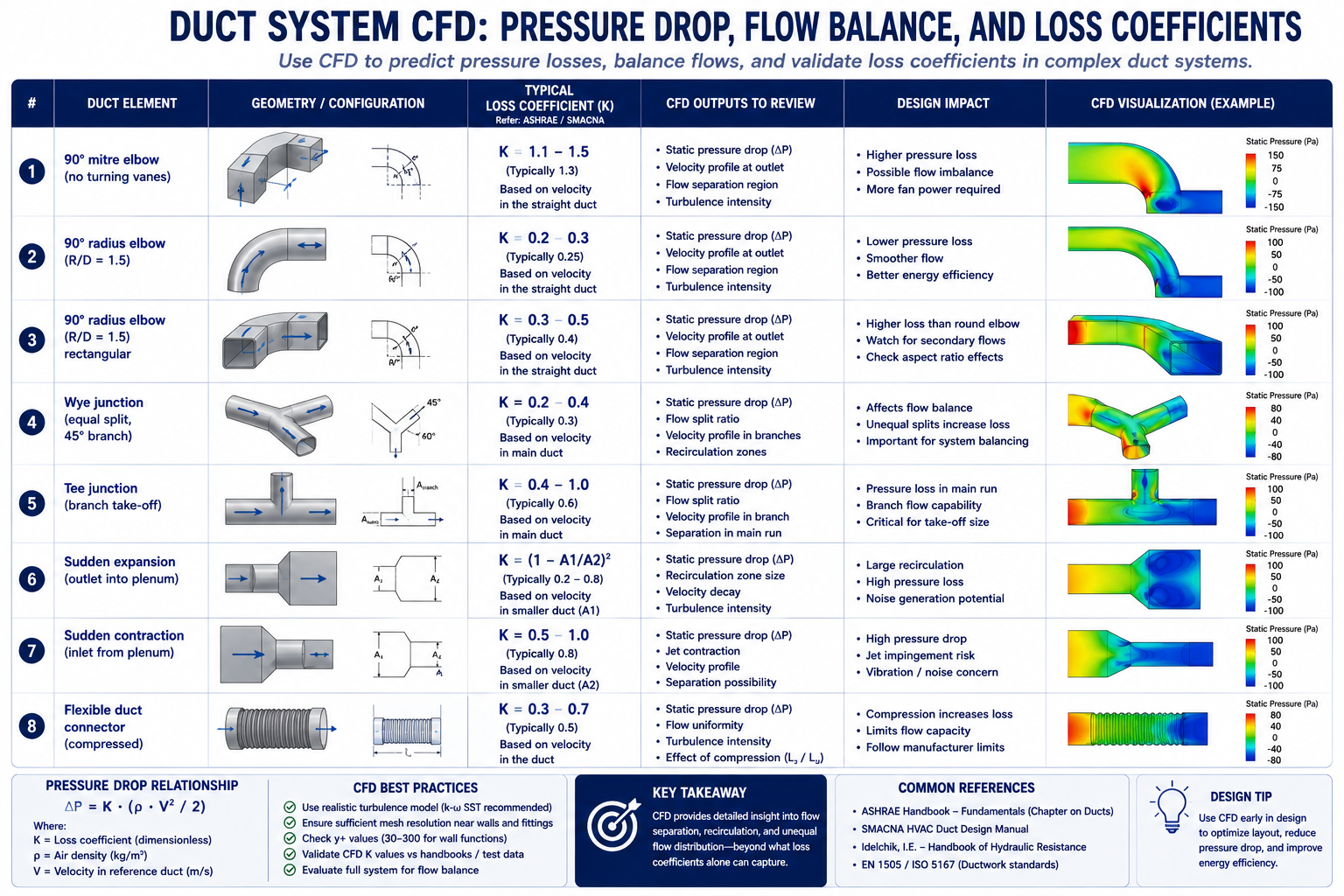
    Duct System CFD: Pressure Drop, Flow Balance, and Loss Coefficients

    Duct systems are commonly designed using the equal friction, static regain, or T-method to size duct sections and estimate pressure losses. These methods rely on tabulated fitting loss coefficients from the ASHRAE Handbook, Fundamentals, Chapter 21, covering elbows, tees, wyes, transitions, and grilles.

    However, these coefficients are based on controlled test conditions and standard fitting geometries. Real duct systems often differ significantly, with rectangular ducts, high aspect ratios, closely spaced fittings, insufficient upstream development lengths, and modified geometries that may not match the available ASHRAE data. In such cases, the tabulated coefficients may not accurately represent the actual airflow and pressure losses.

    CFD fills this gap by computing the actual pressure drop and loss coefficient for the specific fitting geometry in the actual installation condition, including the non-ideal inlet flow profile from the preceding fitting. The table below shows the standard ASHRAE loss coefficients for common duct fittings, the CFD-computed values for the same fittings under typical installation conditions, and the design guidance that CFD reveals.

    Duct System CFD Pressure Drop, Flow Balance, and Loss Coefficients
    Duct ElementLoss Coefficient (C or K)Pressure Drop FormulaCFD vs Standard ValueDesign Guidance
    90° mitre elbow (no turning vanes)C = 1.2–1.5 (based on velocity pressure)ΔP = C × (ρV²/2)CFD: 1.3–1.5; ASHRAE: 1.2; poor agreement for rectangular ductsAvoid mitre elbows, use radius elbows (R/D ≥ 1.5) or add turning vanes
    90° radius elbow (R/D = 1.5)C = 0.11–0.15ΔP = C × (ρV²/2)CFD: 0.12–0.14; ASHRAE: 0.11; good agreement at low turbulence intensityStandard choice for main duct bends; CFD confirms ASHRAE values for round duct
    90° radius elbow (R/D = 1.5) rectangularC = 0.22–0.35 depending on aspect ratioΔP = C × (ρV²/2)CFD reveals 25–40% higher loss than round for same R/D due to secondary flowUse turning vanes for rectangular elbows with aspect ratio > 2:1
    Wye junction (equal split, 45° branch)C_branch = 0.5–0.8; C_straight = 0.1ΔP branch = C × (ρV²/2) of incoming velocityCFD shows strong sensitivity to branch angle and incoming velocity profileEnsure uniform velocity approaching junction; reduce branch angle to 30° to lower C_branch
    Tee junction (branch take-off)C_branch = 0.9–1.5; C_straight = 0.05–0.2Separate C for straight-through and branchCFD critical here, standard C values assume fully developed upstream flowStraight duct of ≥ 10 diameters upstream of tee required for ASHRAE C to be valid
    Sudden expansion (outlet into plenum)C = 1.0 (full dynamic pressure loss)ΔP = ρV²/2 (full velocity pressure)CFD and theory agree well for attached flow; divergence at high expansion ratiosAlways add a grille or diffuser cone at duct exit to duct, avoids full dynamic pressure loss
    Sudden contraction (inlet from plenum)C = 0.5 (typical); 0.04 for well-rounded inletΔP = C × (ρV²/2) of outlet velocityCFD shows vena contracta inside duct; rounding inlet reduces C from 0.5 to < 0.1Round or bell-mouth duct inlets reduce inlet loss by factor of 5+ vs sharp-edged
    Flexible duct connector (compressed)C = 1.5–6.0 depending on compression and bendsΔP = C × (ρV²/2)CFD: highly variable; standard values unreliable for compressed flex ductKeep flex duct fully extended and straight; limit to < 1.8m runs; avoid bends in flex

    Fan Curve Intersection and System Resistance

    The fan operating point is determined by where the fan pressure-flow curve intersects the system resistance curve. If the actual system resistance is higher than expected because of underestimated fitting losses or additional bends, the operating point shifts to lower airflow and higher pressure. As a result, the fan may deliver less airflow than the design requires.

    CFD can evaluate pressure losses using the as-built duct geometry rather than the original design. For example, replacing a radius elbow with a mitre elbow or placing a branch immediately after a bend can significantly increase system resistance. CFD identifies where the additional pressure drop occurs and helps determine whether balancing dampers or duct modifications are needed to restore the required airflow.

    Pressure Balancing in Multi-Branch Systems

    In a multi-branch supply duct system, each branch must deliver its design airflow to maintain proper zone performance. Manual balancing dampers are commonly used during commissioning, but they add resistance to the system and can increase the fan’s energy demand. In poorly designed systems, this additional resistance can account for a significant portion of fan power.

    CFD optimization can improve flow distribution by adjusting branch sizing, tee angles, and junction geometry so that branches achieve more balanced airflow naturally. By iterating the geometry and pressure losses, engineers can reduce reliance on balancing dampers and avoid unnecessary pressure losses. This approach is particularly useful for complex multi-branch systems where conventional calculations cannot fully capture the detailed pressure distribution at junctions.

    Special HVAC Applications: Clean Rooms, Smoke Control, and Data Centres

    Clean Room Airflow: ISO 14644 Compliance Through Simulation

    Clean room HVAC design must comply with ISO 14644-1, which classifies clean rooms by particle count (ISO Class 1 through 9) and specifies the maximum allowable particle concentration at each class. The air distribution system must deliver clean air to the entire work zone without creating turbulent eddies that could carry particles from less-clean regions into the critical process area. ISO 14644-3 specifically accepts CFD as a method for predicting airflow patterns and validating that the specified air change rate and unidirectionality achieve the required cleanliness class before construction

    Cleanroom CFD models typically include the supply HEPA or ULPA filter banks as pressure-drop boundaries, recirculation fan arrays, process equipment as heat sources, operators with metabolic heat output, and low-level return grilles.

    The key output is not simply air velocity, but flow unidirectionality, which shows how consistently the supply air moves in the intended direction, typically downward, without excessive lateral mixing. ISO 14644-3 provides criteria for evaluating airflow characteristics. CFD velocity-vector plots across multiple horizontal and vertical planes can reveal whether unidirectional flow is maintained throughout the critical zone or whether recirculation regions could promote particle accumulation.

    Smoke Control: CFD for Life Safety Compliance

    Smoke control systems in large buildings, atria, underground car parks, shopping centres, airport terminals, must be designed to maintain a clear layer of breathable air below the smoke layer for sufficient time to enable safe evacuation. The performance criteria are defined in fire codes (NFPA 92, BS EN 12101-6, CIBSE Guide E) and typically include: smoke layer height above 2.5 metres from floor level for the first 10 minutes; visibility of at least 10 metres in the clear layer; and CO concentration below 1,500 ppm in the clear layer.

    CFD for smoke control uses tools such as Fire Dynamics Simulator (FDS) or general-purpose CFD with combustion and species-transport models. The simulation represents the fire source, its heat-release rate and growth, the rising thermal plume, smoke-layer development, smoke extraction, and make-up airflows.

    The main output is the smoke-layer height and clear-layer conditions over time, typically from ignition through the first 20 minutes. This helps engineers determine whether the smoke-control system is adequately sized and where modifications may be needed. Unlike analytical models, which are generally limited to simpler geometries, CFD can evaluate smoke movement in complex building layouts.

    Data Centre Hot Aisle/Cold Aisle: CFD as the Primary Design Tool

    Data centre thermal management is a critical CFD application because high-density server racks can generate 10–30 kW of heat within a compact footprint. Cold aisle/hot aisle layouts help manage this heat, but real airflow is more complex than the layout suggests. Cold air can bypass unused rack spaces, hot exhaust can recirculate into cold aisles, and airflow from perforated floor tiles can vary because of underfloor pressure differences.

    CFD models the data hall, server racks, floor tiles, CRAC units, and underfloor plenum to predict these airflow and temperature patterns. The key metric is the server rack inlet temperature, which must remain within the manufacturer’s specified limit at every rack. CFD also identifies hot spots, cold-air bypass, and hot-air recirculation, helping engineers optimize cooling capacity, improve Power Usage Effectiveness (PUE), and maintain sufficient thermal margin for future capacity increases.

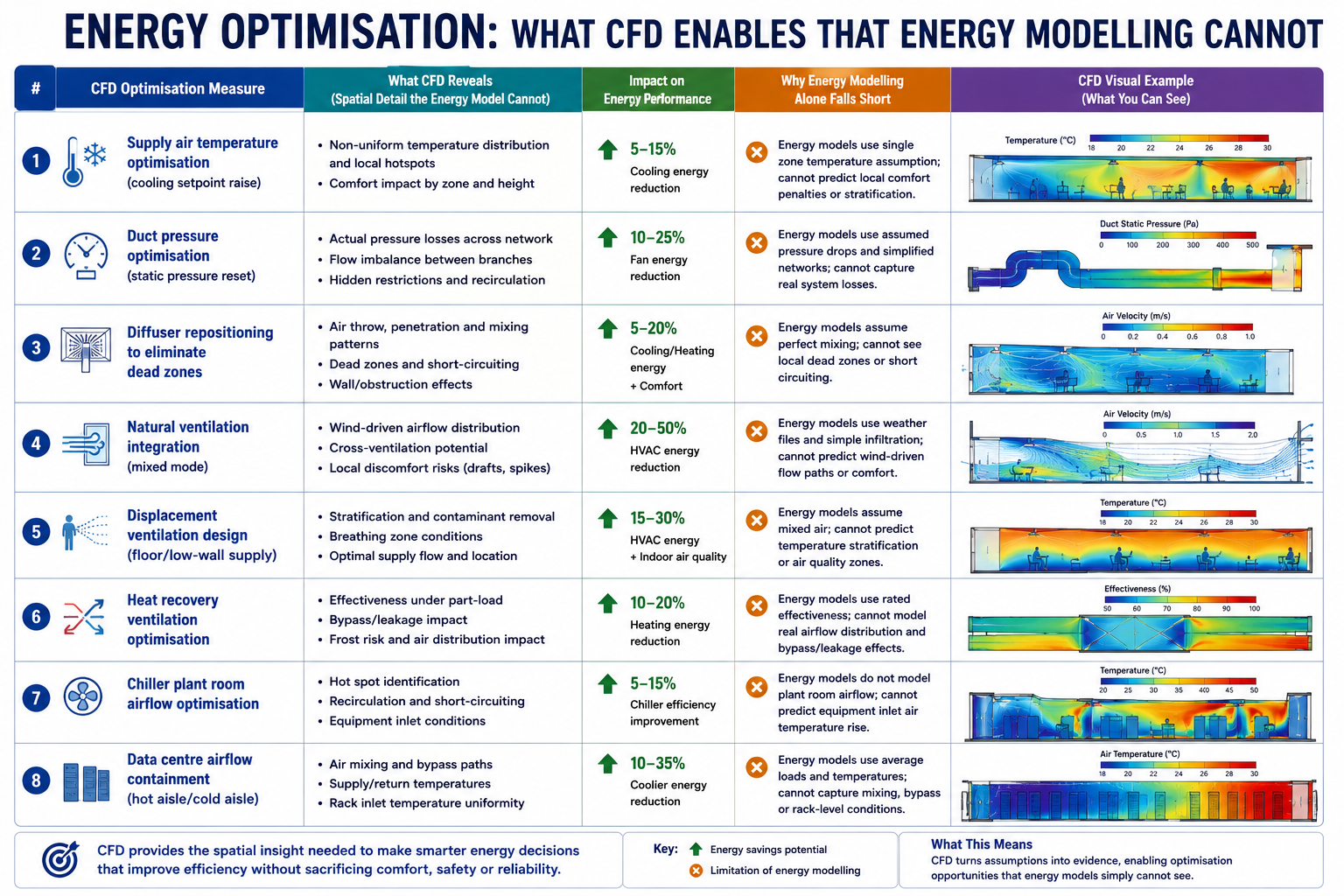
    Energy Optimisation: What CFD Enables That Energy Modelling Cannot

    Building energy modelling tools such as EnergyPlus, IES-VE, and DesignBuilder simulate building thermal loads and HVAC performance hour by hour throughout the year. They are widely used for energy-code compliance and for predicting annual energy use intensity (EUI).

    However, these models typically use simplified, zone-based airflow assumptions and cannot show the detailed airflow distribution within a room. They may therefore be unable to determine whether strategies such as displacement ventilation, natural ventilation, or lower air-change rates can maintain required comfort and indoor air quality. For these decisions, CFD provides the detailed airflow analysis that zone-based energy models cannot.

    Energy Optimisation What CFD Enables That Energy Modelling Cannot

    The energy optimisation measures in the table below are enabled by CFD because each one requires confirming that a changed ventilation strategy, lower airflow, higher supply temperature, different distribution, still meets comfort and indoor air quality criteria. Without CFD, the engineer cannot confirm this and must fall back to conservative assumptions that preserve the original over-designed system

    CFD Optimisation MeasureTypical Energy SavingMechanismPayback PeriodBest Applicable Building Type
    Supply air temperature optimisation (cooling setpoint raise)5–15% cooling energyCFD confirms that raising supply air temperature by 1–2°C while repositioning diffusers maintains comfort, reduced chiller liftImmediate, no capital cost for existing system with variable supply tempOffice, commercial, any VAV system with chiller
    Duct pressure optimisation (static pressure reset)10–25% fan energyCFD identifies over-pressurised branch circuits; static pressure reset reduces fan speed while maintaining all zones at minimum required pressureImmediate for VAV systems with BMS; < 6 months for controls upgradeAny VAV system; largest savings in systems originally set at maximum static pressure
    Diffuser repositioning to eliminate dead zones5–10% ventilation energyCFD identifies under-served zones requiring extra air volume; repositioning diffusers achieves uniform distribution at lower total airflowLow capital; repositioning diffusers costs $200–$2,000 per diffuser depending on ceiling accessOpen-plan offices; retail; spaces with asymmetric occupancy patterns
    Natural ventilation integration (mixed mode)20–50% cooling energy in mild climatesCFD proves operable window positions and stack effect sizing can meet comfort criteria for 40–60% of operating hours, eliminating mechanical cooling3–8 years for window actuator installation; major energy saving for lifetime of buildingOffice, education, residential in temperate climates; not suitable for humid tropical climates without dehumidification
    Displacement ventilation design (floor/low-wall supply)15–30% ventilation fan energy vs overhead mixingCFD validates that lower air change rates achieve same air quality due to ACE > 1.0 for displacement vs 0.8 for mixing, less fan power for same IAQPremium for displacement diffusers vs ceiling diffusers; ROI 3–7 years in energy costsHigh-ceiling spaces: offices, theatres, airports, atriums; not suitable for spaces requiring rapid temperature response
    Heat recovery ventilation optimisation30–50% ventilation heating/cooling energyCFD models cross-contamination risk in heat exchanger bypass conditions; validates minimum outdoor air rates while maximising heat recoveryHeat recovery units: 3–6 years payback in heating-dominated climatesAny building with high ventilation rates: laboratories, schools, hospitals, commercial kitchens
    Chiller plant room airflow optimisation2–8% chiller energyCFD of chiller room reveals recirculation of condenser air; repositioning fans or adding baffles reduces condenser entering air temperature by 1–3°C, improving COPLow capital: baffles $1,000–$10,000; saves 2–5% of chiller energy year-roundAny air-cooled chiller plant; greatest benefit in confined plant rooms with multiple units
    Data centre airflow containment (hot aisle/cold aisle)20–40% cooling energy for data centreCFD quantifies bypass and recirculation flows; hot aisle containment eliminates mixing; supply air temperature can be raised 5–10°C with same server inlet temperature12–24 months typical for hot aisle containment installation in existing data centreData centres and server rooms; any high-density electronics cooling application

    Worked Examples: CFD Driving HVAC Design Changes

    Example 1: Open-Plan Office, Resolving the Dead Zone

    A 400 m² open-plan office floor plate is served by 16 ceiling swirl diffusers at 5m × 5m grid spacing, each supplying 180 L/s at 14°C in cooling mode. The HVAC engineer’s calculation confirmed adequate air change rate (11 ACH) and design throw distance for each diffuser. Post-occupancy surveys showed 28 percent dissatisfaction, concentrated in the two corners farthest from the main supply duct riser.

    CFD model: 3D RANS k-ω SST with buoyancy (Boussinesq approximation); 52 million cell mesh resolving diffuser geometry; steady-state; 26 occupants as heat sources at 75W sensible each; 8 workstation computers at 120W each; perimeter glazing as boundary condition at 35°C surface temperature (peak summer).

    CFD findings: The two corner zones had air velocities below 0.05 m/s and temperatures of 27.5°C, well above the 24°C design point. Mean age of air in the corners was 42 minutes versus 9 minutes (nominal), indicating that only 21 percent of the design air change rate was being achieved in those zones. The failure mode: the corner diffusers were positioned 2.8m from the perimeter wall, within the Coanda attachment zone. The jets attached to the ceiling and ran parallel to the perimeter wall rather than projecting into the room, then short-circuited to return grilles positioned along the corridor.

    CFD-driven design change: Relocate two corner diffusers to 1.2m from the perimeter wall to project jets perpendicular to the glazing, breaking the Coanda attachment and directing air into the unserved zone. Add two additional linear slot diffusers at the perimeter glazing supplying 60 L/s each at 14°C to counteract the solar gain and cold glass convection currents. Reposition one return grille from the corridor side to the interior of the corner zone.

    Predicted outcome from CFD: Corner zone temperatures reduced from 27.5°C to 23.8°C. Air velocity in corner zone increased from 0.05 to 0.12 m/s, below draught threshold. PMV in corner zone improved from +1.4 (warm, 34% dissatisfied) to +0.2 (neutral, 6% dissatisfied). Mean age of air reduced from 42 minutes to 11 minutes. Total supply airflow unchanged, comfort achieved by redistribution, not additional air volume.

    BEFORE (existing diffuser positions):
      Corner zone air temperature:      27.5 °C
      Corner zone air velocity:         0.04–0.06 m/s
      Corner zone CO2:                  1,340 ppm
      Mean age of air (corner):         42 min  (nominal 9 min = 11 ACH)
      Air change effectiveness (ACE):   0.21  (ideal mixing = 1.0)
      PMV corner zone:                  +1.4  (warm)
      PPD corner zone:                  34%   (above 20% threshold)

    AFTER (repositioned diffusers + perimeter slots):
      Corner zone air temperature:      23.8 °C    (-3.7 °C)
      Corner zone air velocity:         0.10–0.13 m/s
      Corner zone CO2:                  870 ppm    (-470 ppm)
      Mean age of air (corner):         11 min     (-31 min)
      Air change effectiveness (ACE):   0.82  (mixing ventilation target = 0.8)
      PMV corner zone:                  +0.2  (neutral)
      PPD corner zone:                  6%    (ASHRAE Class A: < 10%)

    DESIGN COST:
      Diffuser relocation: 2 diffusers moved  ~ $800 labour
      Perimeter linear slots: 2 × 3m runs     ~ $2,400 material + labour
      Duct extension to perimeter slots:       ~ $1,200
      Total remediation cost:                  ~ $4,400

    COMPARISON WITH ALTERNATIVE:
      Increasing total supply airflow by 40% to dilute corner CO2:
        Fan energy increase: +28% (~$3,200/year electricity at $0.15/kWh)
        Does NOT fix temperature non-uniformity or Coanda jet problem
      CFD-guided repositioning achieves better comfort at $4,400 one-time cost
      vs $32,000 ten-year energy cost of the 'more air' alternative

    Example 2: Hospital Operating Theatre, Validating Unidirectional Flow

    A new 36 m² operating theatre is designed with a 3.4 m × 3.4 m HEPA-filtered unidirectional flow (UDF) canopy supplying 0.36 m/s downward air velocity across the surgical site. The theatre also has peripheral low-velocity induction diffusers around the room perimeter. Building regulations (HTM 03-01 in the UK) require that the critical zone around the operating table maintains ISO Class 5 cleanliness (< 3,520 particles ≥ 0.5μm per cubic metre).

    CFD model: 3D RANS; HEPA canopy as uniform velocity inlet; peripheral diffusers as momentum sources; surgical team as heat sources (5 persons at 80W each + 60W metabolic); anaesthetic equipment as obstruction; operating table at body temperature; surgical lights as 400W overhead heat source.

    CFD findings: The unidirectional zone was maintained correctly for 80 percent of the canopy area. However, the anaesthetic screen at the head of the table, a vertical partition 1.2m tall running perpendicular to the airflow, created a recirculation zone on the downstream side. The vortex behind the screen carried particles from the periphery of the theatre back into the lower portion of the UDF zone at the incision site. The contamination risk was highest during patient intubation, when the anaesthetic screen was at its maximum height.

    Design change: Tilt the UDF canopy 3 degrees toward the head of the table to direct the primary jet slightly away from the anaesthetic screen wake. Add two supplementary slot supply points at the head of the table, supplied from the UDF plenum at 0.15 m/s, to fill the recirculation zone behind the screen with clean air. The supplementary slots are integrated into the anaesthetic equipment mounting rail, no additional ceiling penetrations required.

    Outcome: Recirculation zone behind anaesthetic screen eliminated at the incision site level. Particle tracking simulation confirms < 10 particles ≥ 0.5μm per cubic metre at the incision site under worst-case conditions (anaesthetic screen at maximum height, all personnel in position). ISO Class 5 compliance confirmed across the full critical zone. Modification identified before construction, the supplementary slots are built into the equipment rail during factory manufacture at a cost of approximately £800, versus a post-construction modification cost estimated at £15,000 to £25,000 if the problem had been discovered during commissioning testing.

    Example 3: Data Centre, Hot Aisle Containment ROI Analysis

    A 200-rack data centre hall with 2,000m² floor area is operating at average rack power of 6 kW per rack (1,200 kW total IT load). Current cooling configuration uses 12 CRAC units each rated at 150 kW at 18°C supply. The measured average server inlet temperature is 28°C, within specification but with 15 percent of racks showing inlet temperatures above 30°C at peak load. PUE is 1.72.

    CFD findings before containment: Bypass ratio (cold air flowing from cold aisle to hot aisle overhead without passing through racks) was 23 percent of total CRAC supply. Recirculation fraction (hot exhaust air re-entering cold aisle over rack tops) was 18 percent. The combined effect was that 41 percent of cooling capacity was wasted on air that either bypassed the racks or was pre-heated by recirculation before entering the servers.

    CFD model of hot aisle containment: Install full height containment doors at the ends of each hot aisle and a solid ceiling above the hot aisle to the raised floor plenum return. All CRAC units relocated to the hot aisle side to take in the warmest air directly. Supply perforated tiles repositioned to ensure uniform cold aisle pressure.

    CFD Results After Containment

    After hot aisle containment, the bypass ratio decreased from 23% to 3%, while the recirculation fraction dropped from 18% to 2%. Supply air entering the CRAC units increased from an average of 24°C to 34°C, allowing the units to cool directly from the hot aisle rather than a mixed-air environment.

    This made it possible to increase the CRAC supply temperature from 18°C to 23°C while maintaining a server inlet temperature of 28°C. The higher supply temperature improved chiller COP by approximately 18%, contributing to a 24% reduction in cooling energy.

    For a 1,200 kW IT load operating 8,760 hours per year at $0.12/kWh, the improved PUE from 1.72 to 1.42 results in estimated annual savings of approximately $432,000. With a hot aisle containment installation cost of $180,000, the calculated simple payback is about 5 months.

    Building an Accurate HVAC CFD Model: Setup Decisions That Determine Accuracy

    HVAC CFD models have specific setup decisions that differ from structural or external aerodynamics CFD. The following covers the most important HVAC-specific decisions that govern result accuracy.

    Turbulence Model Selection for HVAC

    The RANS k-ω SST model is a common choice for HVAC CFD because it handles wall-bounded flows, supply jets, and room-scale convection at a reasonable computational cost. For typical HVAC temperature differences, the Boussinesq approximation is widely used to model buoyancy. When temperature differences become large or buoyancy dominates, a full variable-density model using the ideal gas law provides greater accuracy.

    The k-ε model is also used for HVAC simulations, but it can be less accurate near walls and in regions with strong flow curvature, such as duct bends and diffuser jets. The SST model combines k-ω behavior near walls with k-ε behavior in the free stream, making it suitable for a broad range of HVAC flow conditions.

    For natural ventilation and low-velocity spaces, where buoyancy-driven flow and thermal stratification dominate, LES or unsteady RANS may be needed to capture transient flow structures. However, these approaches require significantly more computational resources and are generally reserved for research-grade or compliance-critical analyses.

    Diffuser Modelling: The Room Inlet Boundary Condition

    Diffusers are the most challenging element of HVAC CFD because their complex internal geometry, slot vanes, swirl blades, perforated faces, cannot be practically meshed in a room-scale simulation without creating a prohibitively large model. Several simplified approaches are used:

    • Momentum source method (MSM): The diffuser is replaced by a volumetric momentum source in the cells occupying the diffuser location. The source term injects momentum in the correct direction and magnitude to match the diffuser’s throw and spread. Computationally efficient and accurate for the room-scale flow prediction; less accurate near the diffuser itself.
    • Prescribed velocity profile method: A measured or manufacturer-specified velocity profile is applied as an inlet boundary condition at the diffuser face. Requires manufacturer CFD data or physical measurement; more accurate than MSM near the diffuser.
    • Simplified box model: A box representing the diffuser envelope is included in the room geometry, with appropriate inlet faces for the supply slots. Requires fine mesh at the diffuser but correctly predicts the near-diffuser flow pattern including Coanda attachment.

    For most comfort assessment applications, the momentum source method with manufacturer-specified throw characteristics is adequate and is the standard approach in HVAC-specific CFD software (Flovent, Flomerics, Simscale HVAC). For applications where the near-diffuser flow pattern is critical, theatre ventilation, clean room UDF validation, operating theatre compliance, the simplified box or prescribed profile method is preferred.

    Occupant and Equipment Heat Loads

    People and equipment are heat sources that drive the thermal plumes and buoyancy currents that govern room airflow in spaces with moderate to low forced convection. The thermal plume from a seated person (sensible heat output approximately 75W) rises at 0.1 to 0.3 m/s and reaches the ceiling in 3 to 5 seconds in a 3m high room, interacting with the ceiling jet from supply diffusers and creating complex mixed convection patterns that no manual method can predict.

    In HVAC CFD models, people are typically represented as simplified geometry (a seated or standing cylinder or box) with a specified sensible heat flux on the body surface. The exact shape has less influence on the room-scale flow than the heat flux magnitude and the relative positions of people and supply diffusers. Equipment is represented as block geometries with specified heat dissipation rates. For applications where the precise thermal plume from an individual person or workstation matters (operating theatre, clean room, personal comfort ventilation systems), higher-fidelity occupant models with segmented body heat release are used.

    Validating HVAC CFD: When Results Can Be Trusted

    HVAC CFD results are more variable in accuracy than external aerodynamics CFD because the buoyancy-driven flows, diffuser jets, and room-scale turbulence are harder to model correctly than attached boundary layers at cruise conditions. The standard validation approach for HVAC CFD is comparison against ASHRAE Standard 129 benchmark cases, a set of generic room configurations with published experimental data for temperature and velocity distributions that CFD codes can be compared against before being applied to real projects.

    In addition to benchmark case validation, project-specific validation uses one or more of the following:

    1. Air temperature measurement: Calibrated temperature sensors at standardised heights (0.1m, 0.6m, 1.1m, 1.7m above floor per ASHRAE 55) at multiple room locations. CFD predictions within ±1.5°C of measured values are considered good agreement for room temperature. Large discrepancies (> 3°C) indicate errors in supply air conditions, thermal load estimates, or diffuser modelling.
    2. Air velocity measurement: Omnidirectional anemometers at occupied zone locations. Agreement within ±0.05 m/s or 20 percent of measured velocity (whichever is larger) is typical for HVAC CFD. High-velocity regions near diffusers require accurate diffuser modelling for velocity agreement.
    3. CO2 tracer gas: SF6 or CO2 tracer gas injected at the supply and measured at multiple return and room locations. The tracer gas concentration distribution validates the CFD-computed flow distribution and age-of-air predictions. This is the most sensitive validation for ventilation effectiveness, concentration non-uniformities that temperature measurements miss are revealed by tracer gas.
    4. Smoke visualisation: Theatrical smoke or titanium tetrachloride smoke bombs reveal the actual flow pattern in a room, showing jet directions, recirculation zones, and dead zones. Not quantitative but provides immediate qualitative confirmation of the CFD-predicted flow pattern, or reveals patterns that the CFD model did not predict, indicating modelling errors to correct.

    Frequently Asked Questions

    Q: Can CFD replace manual HVAC design calculations?

    No. CFD complements manual HVAC calculations rather than replacing them. Manual methods determine loads, airflow, duct sizing, pressure drops, and equipment selection, while CFD evaluates how air actually moves through the space, including temperature distribution, occupant comfort, and draught risk. The best approach is to use manual calculations for system sizing and CFD for airflow distribution validation and optimization.

    Q: What is the Coanda effect and why does it matter for HVAC diffuser design?

    The Coanda effect causes a fluid jet to remain attached to a nearby surface. In HVAC, ceiling-mounted supply jets can attach to the ceiling and travel farther across the room before dropping into the occupied zone, helping reduce draughts. However, excessive attachment can carry the jet past its intended path and cause short-circuiting or dead zones near return grilles and perimeter walls. CFD can predict how jet momentum, supply temperature, and ceiling geometry affect Coanda attachment and detachment, which simplified throw-distance calculations cannot fully capture.

    Q: How does CFD help with HVAC energy optimisation?

    CFD enables HVAC energy optimization by confirming that lower-energy operating strategies still meet thermal comfort and indoor air quality requirements. For example, raising supply air temperature from 13°C to 16°C can improve chiller efficiency, but it also changes jet buoyancy, Coanda attachment, and occupied-zone temperature distribution. CFD can verify whether comfort is maintained before the change is implemented. If the criteria are met, the higher setpoint can reduce cooling energy without major capital changes.

    Q: What is air change effectiveness and how does CFD compute it?

    Air change effectiveness (ACE) measures how effectively fresh supply air reaches the occupied zone. An ACE of 1.0 represents ideal mixing, while values above 1.0 indicate more effective air delivery, such as displacement ventilation. Values below 1.0 indicate poor distribution or short-circuiting between supply and return air.

    CFD calculates ACE by tracking the age of air throughout the room using an additional transport equation. This provides the local and zone-average air age and shows where fresh air reaches occupants efficiently or where it is bypassing the occupied zone. Because ACE depends on the full three-dimensional airflow field, it cannot be accurately determined from conventional manual HVAC calculations alone.

    Q: How accurate is HVAC CFD compared to physical measurement?

    HVAC CFD accuracy depends on the application and model quality. For forced-convection rooms, temperature predictions are typically within ±1.5–3°C and occupied-zone velocity within ±0.03–0.08 m/s of measurements. Naturally ventilated spaces can have larger temperature errors of ±3–5°C, while CO₂ predictions are typically within 10–20% when airflow distribution is accurately captured. For code compliance, CFD should be validated against benchmark data or physical measurements.

    Q: When is HVAC CFD required rather than just beneficial?

    HVAC CFD becomes essential in four situations: regulatory compliance for applications such as operating theatres, smoke control, and cleanrooms; complex or non-standard geometries such as atria and large open halls; mixed-mode or natural ventilation, where wind and buoyancy-driven flows interact; and post-occupancy problems, where CFD can identify airflow deficiencies in an as-built system and guide targeted corrective measures instead of trial-and-error adjustments.

    Conclusion: CFD as the Design Verification Tool for HVAC Performance

    HVAC systems can be correctly sized using established manual calculation methods, yet still fail to perform as expected when supply air does not reach occupants at the right quantity, temperature, and velocity. The actual distribution of airflow and temperature depends on three-dimensional effects such as Coanda attachment, buoyancy plumes, furniture and partitions, and supply-to-return short-circuiting. CFD captures these effects and can identify comfort problems, CO₂ accumulation, inadequate diffuser throw, and airflow deficiencies before commissioning. This makes CFD particularly valuable when air distribution directly affects building performance and occupant comfort.

    The strongest approach is to use manual calculations for HVAC system sizing and CFD for airflow distribution validation and optimization. CFD can also support energy-saving strategies such as higher supply temperatures, lower air-change rates, displacement ventilation, and hot aisle containment. By identifying problems and testing design changes before construction or commissioning, CFD can reduce costly remediation, improve occupant comfort, and help HVAC systems perform as designed from day one.

    Explore related simulation topics: thermal simulation in electronics, CFD vs wind tunnel testing, static vs dynamic analysis, why simulation fails, and how leading industries deploy simulation to improve performance and reduce cost.

  • CFD vs Wind Tunnel Testing: Which Is Better? (With Decision Table)

    CFD vs Wind Tunnel Testing: Which Is Better? (With Decision Table)

    In 2019, the aerodynamics team at a major automotive OEM compared the drag coefficient predictions from their CFD model against their full-scale wind tunnel measurement for the same production vehicle. The CFD result was 0.273. The tunnel result was 0.281. The eight drag-count difference, 0.008 Cd, represented approximately 0.8 percent additional fuel consumption at highway speed, translating to roughly 0.15 liters per 100 km across the fleet. Across 200,000 vehicles produced annually, over a 10-year vehicle life, that eight drag-count discrepancy was worth approximately $180 million in fuel cost to their customers.

    The question was not whether CFD or the tunnel was ‘better’, both were used. The question was which result to trust for homologation and which to use for design exploration.

    That question, which method to trust for which decision, is what the CFD vs wind tunnel debate is actually about. Not a competition between two methods, but a decision framework for deploying each where it delivers the most value. CFD and wind tunnel testing are not substitutes for each other in any demanding aerodynamic application. They are complementary tools with different strengths, different limitations, different costs, and different appropriate use cases. Understanding the technical basis of those differences, not just the intuitive ones, but the specific error sources, accuracy ranges, and conditions where each method fails, is the prerequisite for making correct deployment decisions.

    This article provides that technical basis: the complete 12-parameter comparison table, the turbulence model hierarchy and its accuracy boundaries, the seven wind tunnel correction factors and their magnitudes, the Reynolds number problem that each method handles differently, and the 12-case decision table that maps specific applications to the recommended primary and secondary methods with justification. The article also addresses the increasingly important question of CFD validation against tunnel data, how to build a CFD model that can be trusted for extrapolation beyond the test conditions, and what level of agreement between CFD and tunnel constitutes adequate validation.

    What Each Method Actually Measures

    Before comparing the two methods, it is essential to understand what each one fundamentally does, because they are not measuring or predicting the same thing in the same way, and this asymmetry drives most of the nuance in the comparison.

    CFD vs Wind Tunnel, The Cost-Accuracy-Speed Triangle A triangular diagram with three vertices labeled COST (bottom left), ACCURACY (bottom right), and SPEED (top). Three positions are marked on the triangle: Wind Tunnel sits close to the ACCURACY vertex (high accuracy, high cost, slow); RANS CFD sits close to the SPEED vertex (fast, low cost, moderate accuracy for attached flow, poor for separated); LES/DES CFD sits in the center-right area (high cost, slow, high accuracy). Arrows from each position to the vertices show the trade-off profile. A second overlay shows the industry application bands: aviation certification zone close to the tunnel position; early-stage design exploration zone close to RANS; final performance verification zone between RANS and LES. Color coding: tunnel in navy, RANS in light blue, LES/DES in teal. A note at the bottom: 'There is no single best method, the optimal choice depends on which vertex of the triangle the application prioritizes

    A wind tunnel test measures the integrated aerodynamic forces and moments on a physical model in a controlled flow environment. The fluid is real. The turbulence is real. The boundary layer transition from laminar to turbulent flow happens as it would in nature, at the Reynolds number of the test (which may or may not match the full-scale Reynolds number, more on this below).

    The measurement instruments, force balances, pressure taps, particle image velocimetry (PIV) systems, hot-wire anemometers, have measurement uncertainty, calibration drift, and installation effects that must be quantified and corrected. The tunnel itself has walls, a model support structure, and a boundary layer growing on its walls, all of which affect the flow around the model in ways that must be corrected before the data represents free-air conditions.

    A CFD simulation solves the Navier-Stokes equations numerically for a mathematical model of the fluid domain. The governing equations are exact, they correctly describe fluid motion at any Reynolds number, including turbulent flow. The problem is that solving them exactly (Direct Numerical Simulation) requires resolving every turbulent eddy down to the Kolmogorov scale, which at engineering Reynolds numbers would require computational meshes of 10¹² to 10¹⁶ elements and thousands of years of compute time on current hardware.

    Every practical CFD method approximates the turbulence: RANS models time-average the equations and model all turbulence effects; LES models resolve large eddies and model only small eddies; DES uses RANS near walls and LES in separated regions. The approximation introduces modeling uncertainty that is the fundamental limitation of CFD accuracy.

    The Fundamental Asymmetry: Modeling vs Measurement Uncertainty

    This leads to the fundamental asymmetry between the two methods. Wind tunnel tests have measurement uncertainty, errors in the instruments, the corrections, and the test conditions, but they measure real fluid behavior. CFD has modeling uncertainty, errors in the turbulence model approximations, the boundary condition assumptions, and the numerical discretization, but given a correct model, it predicts the full flow field at every point in the domain.

    The practical consequence: wind tunnel results are more trustworthy for configurations where CFD modeling uncertainty is large (massively separated flow, high angle of attack, complex turbulent wake structures) but less useful for configurations where measurement corrections are large and uncertain (very high Reynolds number, novel geometry with no correction calibration data, aeroelastic deformation). CFD is more trustworthy for configurations where the physics is well-captured by RANS (attached flow at cruise conditions, internal pipe flow, HVAC) and where parametric variation is needed that would be too expensive to test physically.

    CFD vs Wind Tunnel: The 12-Parameter Comparison

    The following table provides a structured comparison across twelve parameters that determine which method is appropriate for a given application. The ‘Verdict’ column identifies which method has the advantage for each parameter, but note that no single method wins on all parameters, which is why both continue to be used in demanding aerodynamic programs.

    ParameterCFDWind Tunnel TestingVerdict
    Cost per test/run$500–$5,000 per simulation run (compute + analyst time); large RANS runs $2,000–$10,000; LES/DES $10,000–$100,000+$20,000–$500,000 per wind tunnel entry; model fabrication $50,000–$500,000 additional for complex scale modelsCFD wins for parametric studies; tunnel wins for single definitive result on complex geometry
    Setup timeCAD to first result: 1–5 days for RANS; 1–4 weeks for high-fidelity LES/DESModel fabrication: 4–16 weeks; tunnel booking lead time: 4–26 weeks at major facilitiesCFD wins decisively, weeks vs months
    Design iteration speedGeometry change to new result: hours to days; automated parametric sweeps possibleEach geometry change requires model modification or new model build: weeks per iterationCFD wins, orders of magnitude faster iteration
    Physical realismDepends entirely on turbulence model choice; RANS misses separated flow; LES captures more physics at high costReal fluid at real Reynolds number (if correctly scaled); no turbulence modelling assumptionsWind tunnel wins for complex separated flows and high-Re regimes where turbulence models are uncertain
    Reynolds number matchingFull-scale Re achievable at any geometry size; no scaling requiredRequires pressurized tunnel, cryogenic tunnel, or geometric scaling to match Re, expensive or limitedCFD wins, exact Re matching is trivial
    Measurement completenessFull-field data: pressure, velocity, temperature, turbulence quantities at every point in the domainPoint measurements (pressure taps, hot wires); limited field measurements (PIV); no internal flow data without probesCFD wins for full-field insight; tunnel wins for boundary layer detail
    Accuracy for attached flow (low angle of attack)RANS within 1–5% of measured drag and lift for well-attached flow; excellent for cruise conditionsDirectly measures forces and moments; gold standard for attached flow aerodynamicsTunnel wins or ties, RANS is accurate here but tunnel has no modeling uncertainty
    Accuracy for separated/turbulent flowRANS significantly over-predicts separation; LES/DES accurate but expensive; fundamental modeling uncertainty remainsMeasures actual separated flow if Re is correctly matched; no turbulence model uncertaintyTunnel wins, RANS is unreliable for separated flow; only LES/DES approaches tunnel quality
    Multi-physics couplingFluid-structure interaction, aero-acoustic, conjugate heat transfer available in same frameworkStructural response requires separate instrumentation; acoustics measured separately; heat transfer limitedCFD wins, integrated multi-physics analysis
    Regulatory acceptanceAccepted in many industries as primary method or supplement; required by some codes (wind engineering, CFD for novel aircraft); not universally accepted for certificationGold standard for aerospace certification (FAA AC 25.1); required for final drag polar in commercial aviationTunnel required for aviation certification; CFD accepted in most other industries
    Intellectual property riskGeometry stays in-house; no external exposureScale model sent to test facility; contractor has access to proprietary geometryCFD wins for IP-sensitive programs
    Uncertainty quantificationGrid study, model sensitivity, boundary condition sensitivity quantifiable systematicallyTunnel correction factors (blockage, wall interference, model support) introduce uncertainty that is difficult to fully quantifyCFD provides more systematic uncertainty pathway; tunnel corrections are empirical

    The Turbulence Modeling Problem: Why CFD Accuracy Is Flow-Dependent

    The accuracy of CFD for aerodynamic prediction is not a fixed number, it is a strong function of the flow regime, specifically of how much turbulent separation is present. For fully attached flow at cruise conditions, the flow regime that governs fuel efficiency in commercial aviation and highway aerodynamics for cars, RANS CFD is highly accurate, typically predicting lift and drag within 3 to 5 percent of tunnel measurement. For massively separated flow, bluff bodies, high angle of attack, post-stall aerodynamics, RANS CFD fails systematically and significantly, over-predicting attached regions and under-predicting wake size. Understanding which turbulence model to use, and when RANS is fundamentally inadequate, is the central technical competency for CFD aerodynamics work.

    ModelFull NameComputational CostAccuracy for Attached FlowAccuracy for Separated FlowTypical Use Case
    RANS k-εReynolds-Averaged Navier-Stokes, k-epsilon closureLow (1x baseline)Good, within 3–5% for drag and lift at low AoAPoor, over-predicts separation, under-predicts wake widthExternal aerodynamics at cruise; HVAC; pipe flow; early design exploration
    RANS k-ω SSTk-omega Shear Stress TransportLow (1.1x)Very good, better near-wall behaviour than k-ε; standard for aerodynamicsModerate, better than k-ε for mild separation; still unreliable for massively separated flowAutomotive aerodynamics; aircraft cruise; most industrial external flow
    RANS Spalart-AllmarasOne-equation RANSVery low (0.8x)Good for attached boundary layers; standard in aerospace RANSPoor for separated flow, single equation cannot capture complex turbulenceAerospace RANS (primary model in NASA CFD); thin airfoil attached flow
    DESDetached Eddy SimulationHigh (10–50x RANS)Good, RANS near walls, LES in separated regionsGood, captures unsteady separated flow that RANS misses; time-averaged results competitive with tunnelHigh-AoA aerodynamics; bluff body flows; automotive separated wake
    LESLarge Eddy SimulationVery high (100–1000x RANS)Excellent, resolves large turbulent structures directlyExcellent, captures unsteady separated flow, wake dynamics, acoustic sourcesAeroacoustics; fundamental turbulence research; complex separated flows where DES is insufficient
    DNSDirect Numerical SimulationProhibitive (10^6–10^9x RANS)Exact, resolves all scales of turbulenceExact, no turbulence modellingLow-Re academic research only; not used in industrial aerodynamics

    Why RANS Fails for Separated Flow

    Reynolds-Averaged Navier-Stokes (RANS) models work by time-averaging the Navier-Stokes equations and representing the effect of turbulent fluctuations through a turbulent viscosity, an additional viscous-like term that smears out the turbulent mixing. This works well for attached turbulent boundary layers, where the turbulence is reasonably well described by a local equilibrium between production and dissipation of turbulent kinetic energy. It fails for separated shear layers, where the turbulence is far from local equilibrium, where large unsteady vortex structures shed periodically, and where the flow field is inherently three-dimensional and time-dependent.

    The specific failure mode of RANS in separated flow is reattachment prediction. RANS models systematically predict that separated flow will reattach to the surface earlier than it does in reality, producing a smaller separation bubble, a narrower wake, and lower drag than the physical flow. For a bluff body (a truck, a building, a high-angle-of-attack wing), RANS under-predicts drag by 10 to 30 percent because it predicts a narrower, more rapidly reattaching wake than actually exists. This is not a mesh density problem, refining the RANS mesh does not fix this error, because the error is in the turbulence model, not in the numerical discretization.

    The solution is scale-resolving simulation: DES (which switches from RANS near walls to LES in separated regions) or full LES (which resolves large turbulent eddies directly and models only the small ones). These methods capture the unsteady large-scale vortex shedding that RANS time-averages away, producing time-accurate predictions of the separated flow that, when averaged over sufficient time, agree with tunnel measurements to within 5 to 10 percent for bluff body drag. The cost is 10 to 100 times higher compute time than RANS, but for applications where separated flow governs the answer, it is the only CFD path to reliable results.

    The k-ω SST Model: Why It Became the Industrial Standard

    The k-omega Shear Stress Transport (SST) model, developed by Florian Menter at NASA in 1993, has become the default turbulence model for industrial aerodynamics CFD. Its dominance is not accidental: SST combines the strengths of two earlier models, the k-ε model’s robustness in the freestream and the k-ω model’s superior near-wall behavior, through a blending function that transitions between them based on distance from the wall.

    For attached and mildly separated flows, SST consistently outperforms both k-ε and Spalart-Allmaras across a wide range of geometries and flow conditions. It is not the most accurate model for any specific flow type, but it is the most consistently reliable across the range of conditions found in a typical aerodynamic design campaign. For automotive external aerodynamics, where the flow is moderately separated in the near-wake but attached elsewhere, SST is the standard choice at major OEMs and is accepted by regulatory bodies (homologation wind tunnel standards) as a valid CFD methodology when properly validated.

    Wind Tunnel Limitations: The Corrections That Make Raw Data Unreliable

    Wind tunnels are not perfect simulators of free-air flight or driving conditions. Every wind tunnel test requires a set of data corrections to convert the raw measurements into values that represent the aerodynamic performance of the full-scale vehicle or structure in free air. These corrections are based on analytical models, empirical data, and tunnel-specific calibration constants that introduce their own uncertainty. Understanding the magnitude and uncertainty of wind tunnel corrections is essential for correctly interpreting tunnel data and for understanding why ‘tunnel data’ is not the same as ‘truth data’.

    Wind Tunnel Limitations
    Correction TypePhysical CauseTypical MagnitudeEffect if UncorrectedStandard Method
    Solid blockageModel frontal area displaces streamlines, increasing local velocity above freestream0.5–5% velocity increase for blockage ratio 0.5–5%Drag and lift overestimated; results not representative of free-air conditionsMaskell or Thom method based on model frontal area / test section area ratio
    Wake blockageModel wake displaces streamlines, further accelerating flow around model0.5–3% additional to solid blockageAdditional drag overestimation; particularly significant for bluff bodies with large wakesCombined with solid blockage in Maskell method; or experimental with empty tunnel reference
    Streamline curvature (buoyancy)Longitudinal pressure gradient in tunnel due to growing boundary layer causes apparent drag increase0.5–2% drag correction for large tunnels; larger in smaller facilitiesDrag overestimated; effect proportional to model length relative to tunnel lengthHorizontal buoyancy correction using measured axial pressure gradient
    Wall interference (lift)Tunnel walls constrain wing tip vortices, reducing induced downwash below free-air value; lift slope increased1–5% lift correction for typical aircraft models; larger for high-span modelsEffective angle of attack and induced drag not representative of free air; lift curve slope too steepPrandtl-Glauert correction or panel method wall interference calculation from wall pressure measurements
    Model support interferenceSting, strut, or wire support system adds its own aerodynamic force to measured model force1–10% drag interference; difficult to quantify preciselyDrag and pitching moment contaminated by support aerodynamicsDummy sting/strut test to quantify support interference; subtract from model result
    Reynolds number mismatchModel tested at lower Re than full-scale; boundary layer transition location differs; skin friction drag different1–15% drag error depending on Re ratio and surface roughness treatmentDrag polar, stall angle, and maximum lift significantly different from full-scale if transition not correctly matchedBoundary layer trip (roughness strip) to force transition at model location; Re correction factor
    Model deformation under loadAerodynamic loads bend wing models; deformed shape is what the tunnel sees, not the design shapeWing twist up to 1–2 degrees for typical structural models under full loadAeroelastic deformation changes effective incidence; lift distribution differs from rigid model assumptionOptical measurement of model deformation under load; correct aerodynamic data to zero-load shape

    The Reynolds Number Problem: Scale Models and Real Conditions

    The most fundamental limitation of wind tunnel testing is the Reynolds number scaling problem. The Reynolds number Re = rho*V*L/mu governs the ratio of inertial to viscous forces in a flow. Two flows at the same Reynolds number are dynamically similar, they have the same non-dimensional flow structure regardless of the actual velocities and length scales. A scale model tested at the correct Reynolds number produces aerodynamic coefficients that correctly represent the full-scale vehicle.

    The problem: for a 1/4-scale model to match the full-scale Reynolds number, the tunnel airspeed must be four times the full-scale speed. For a commercial aircraft cruising at 250 m/s (Mach 0.85), the 1/4-scale model would need to be tested at 1,000 m/s, well above the speed of sound, completely changing the compressibility effects.

    Solutions exist but are expensive: pressurized tunnels increase air density to raise Re at the same velocity (NASA’s National Transonic Facility and ETW in Cologne operate at up to 9 atmospheres); cryogenic tunnels reduce air viscosity by cooling to -170°C, raising Re for the same speed (ETW operates at both pressure and cryogenic conditions simultaneously, achieving full-scale Re for large aircraft models). Both approaches add significant cost and operational complexity to testing.

    CFD has no Reynolds number scaling problem. A CFD simulation runs at exactly the full-scale Reynolds number regardless of the geometry scale, the mesh simply needs to resolve the boundary layer at the actual flow conditions. This is one of CFD’s clearest advantages over wind tunnel testing: the simulation represents the actual vehicle at the actual operating condition, with no scaling uncertainty to correct for.

    The Model Support Interference Problem

    Every wind tunnel model must be supported in the tunnel by some structure, a sting attached to the model base and supported by a central strut, side struts, wires, or a floor-mounted support. Each support structure creates its own aerodynamic disturbance that contaminates the measurement: the sting interferes with the base pressure, the struts interfere with the wing tip flow or the fuselage boundary layer, and the wake of the support structure interacts with the model wake.

    The standard approach to quantifying support interference is the dummy support test: a mirror-image of the support structure is installed in the tunnel without a model attached, and its aerodynamic force is measured. This force is then subtracted from the model-plus-support measurement to give the isolated model result. This approach works reasonably well for simple support geometries but cannot account for the mutual aerodynamic interference between the support and the model, the way the presence of the support changes the flow around the model and vice versa. This mutual interference is particularly significant for rear-steer and sting-supported aircraft models where the sting enters the model base in the middle of the wake region that governs base drag.

    CFD Validation Against Wind Tunnel Data: Building Trustworthy Simulations

    CFD validation, comparing simulation predictions against trusted experimental measurements, is the process by which a CFD model earns the right to be used for design decisions beyond the tested configuration. A CFD model that has not been validated is not yet a reliable tool; it may produce accurate results or inaccurate results for any new geometry, and there is no basis for distinguishing between the two without the reference data that validation provides.

    The AIAA Guide for Verification and Validation of CFD Simulations (AIAA G-077) and the ASME V&V 20 standard define the framework for CFD validation: the simulation is validated when its predictions agree with experimental measurements within a defined uncertainty band that accounts for both simulation uncertainty and experimental measurement uncertainty. If the simulation and experiment disagree by more than the combined uncertainty, there is a validation failure, either the simulation has a model error, the experiment has an unquantified systematic error, or both.

    Computational Fluid Dynamics (CFD) enables engineers to evaluate multiple wind-loading scenarios by modifying simulation parameters without rebuilding physical models. This makes CFD especially valuable during the early design stage, where rapid design iteration and optimization are important.

    DLUBAL

    What Good CFD-Tunnel Correlation Looks Like

    For attached flow aerodynamics at cruise conditions (the primary design regime for commercial aircraft and highway vehicle aerodynamics), good CFD-tunnel correlation is defined as:

    • Drag coefficient (Cd): CFD within 5 drag counts (0.0005 Cd) of tunnel measurement for well-attached flow; within 10 drag counts for mild separation regions. One drag count = 0.0001 in Cd, representing approximately 0.1% fuel consumption for a commercial aircraft.
    • Lift coefficient (Cl): CFD within 1–2% of tunnel measurement at matched angle of attack for attached flow. Lift prediction is generally more accurate than drag prediction because lift is dominated by pressure integration over the wing, which RANS captures well.
    • Surface pressure distribution (Cp): CFD Cp values within 0.02–0.05 Cp units of tunnel pressure tap measurements along the span and chord. Large local Cp discrepancies (> 0.1) indicate regions of flow separation or transition behavior that the CFD model is not capturing correctly.
    • Pitching moment (Cm): CFD within 0.005–0.01 Cm units of tunnel measurement. Moment prediction is more sensitive to the aft-loading distribution and is a more demanding validation criterion than lift.

    For separated flow at high angle of attack or bluff body geometries, these criteria are relaxed: drag within 10–20%, lift within 5%, and the requirement is primarily that the CFD captures the correct physical mechanism, the correct location of separation, the correct wake width, the correct vortex shedding frequency, rather than achieving the same numerical precision as for attached flow.

    When CFD Disagrees With the Tunnel: Diagnostic Protocol

    When CFD predictions and tunnel measurements disagree beyond the accepted uncertainty band, the investigation must determine whether the discrepancy reflects a CFD model error, a tunnel measurement error, or a condition mismatch (different Reynolds number, different turbulence intensity, different model geometry than the CFD). The diagnostic protocol:

    1. Check condition matching: Confirm that the CFD boundary conditions exactly match the tunnel test conditions: freestream velocity, Reynolds number, angle of attack, Mach number (if compressible), and turbulence intensity at the inlet. Even 0.1-degree angle of attack mismatch produces measurable Cl and Cm discrepancy.
    2. Compare surface pressure distributions, not just integrated forces: If Cd disagrees, compare Cp distributions along the chord at several spanwise stations. If Cp agrees locally but the integrated Cd does not, the discrepancy is in the tunnel corrections (blockage, wake survey). If Cp disagrees locally, the CFD is not predicting the correct flow physics at those locations.
    3. Check tunnel corrections: Review each correction factor applied to the raw tunnel data. Blockage corrections are the most common source of systematic offset between CFD and tunnel. A 3% blockage with a 10% overcorrection produces a 0.3% drag bias, several drag counts that appear as a CFD error but are actually a tunnel data processing error.
    4. Test mesh sensitivity: Run a grid refinement study, coarse, medium, fine mesh, and confirm that the CFD result has converged. If the result is still changing with mesh refinement, the discretization error is contributing to the discrepancy and must be eliminated before comparing with tunnel data.
    5. Test turbulence model sensitivity: Run the same geometry with two or three turbulence models (SST, Spalart-Allmaras, Realizable k-ε) and compare. If the models agree but disagree with the tunnel, the discrepancy is unlikely to be a turbulence modeling error, look to the tunnel corrections or condition mismatch. If the models disagree with each other and one agrees with the tunnel, the turbulence model sensitivity is the primary source of CFD uncertainty.

    Cost, Time, and Infrastructure: The Practical Realities

    Wind Tunnel Costs: Entry Fees, Model Costs, and Lead Times

    The cost of a wind tunnel test program has three major components: tunnel rental, model fabrication, and data acquisition and analysis staffing. Tunnel rental rates at major facilities range from $5,000 to $50,000 per shift (8 hours) depending on tunnel size, capability (subsonic vs transonic vs supersonic), and facility prestige. A full aerodynamic development program for a commercial aircraft at a major transonic tunnel (NASA Ames, DNW, ONERA S1MA) requires 4 to 12 weeks of tunnel time over 2 to 3 entries, totaling $2 million to $15 million in tunnel costs alone.

    Model fabrication is often the larger cost. A high-quality 1/6-scale aircraft model with a full complement of pressure taps (1,000 to 5,000 taps), a force/moment balance, and a remotely actuated control system costs $500,000 to $3 million to design and build. The model must withstand the aerodynamic loads at maximum tunnel dynamic pressure, typically requiring high-strength steel or aluminum construction with carefully machined surfaces to sub-millimeter accuracy. Model fabrication lead time is typically 12 to 24 months for a complex aircraft model, representing a program schedule commitment that cannot be easily shortened.

    In contrast, a CFD simulation setup and run for the same geometry, once the CAD model exists, takes days to weeks. A production-quality RANS analysis of a full aircraft at cruise takes 2 to 5 days of setup and 4 to 24 hours of compute time on a 64-to-256-core cluster, at a total cost of $1,000 to $10,000 including compute and analyst time. A CFD team can run as many geometry variations as engineering judgment requires, at marginal cost per run, versus a tunnel team that must commit to the model geometry 12 to 24 months before testing.

    The Hidden Costs of Each Method

    Both methods have hidden costs that are not immediately obvious from headline prices. For wind tunnels, the hidden costs are: model modification costs (changing a surface contour or control surface on a tunnel model requires machining new parts and reassembling, typically $20,000 to $100,000 per modification and 2 to 4 weeks of lead time), tunnel correction uncertainty (the cost of acting on results that were later found to have uncorrected systematic errors in the tunnel data), and schedule risk (the cost of program delay when a tunnel entry reveals a performance shortfall that requires a design change cycle before the next entry).

    For CFD, the hidden costs are: validation cost (CFD without tunnel validation is of uncertain reliability for design decisions, the cost of the tunnel program used to validate the CFD model must be allocated to the CFD program’s total cost), compute infrastructure (a serious CFD program requires HPC clusters costing $500,000 to $5 million, with ongoing power, cooling, and maintenance costs), and expert analyst time (high-fidelity CFD is not a push-button technology, experienced CFD engineers at $150,000 to $250,000 per year in total compensation are the primary operational cost of a CFD program).

    Decision Table: CFD vs Wind Tunnel for 12 Applications

    The following table maps 12 common aerodynamic applications to the recommended primary method, the role of the secondary method, and the rationale for each decision. Use this table as the starting point for method selection, the rationale column identifies the specific technical or regulatory driver for each recommendation.

    Decision Table: CFD vs Wind Tunnel for 12 Applications
    ApplicationRecommended Primary MethodRole of Secondary MethodRationale
    Commercial aircraft cruise drag polarWind tunnel (low-speed + high-speed transonic)CFD for parametric geometry exploration before tunnel entry; post-tunnel CFD extrapolationFAA certification requires tunnel validation; drag count accuracy (1 drag count = 0.1% fuel burn) requires tunnel precision
    Automotive drag coefficient (Cd) developmentCFD (RANS k-ω SST) for parametric sweep; tunnel for final confirmationTunnel for final Cd validation and surface pressure measurement correlationAutomotive schedules require fast iteration; tunnel used for model validation and regulatory homologation data
    Formula 1 / motorsport aerodynamicsCFD and tunnel in parallel (FIA regulated hours of both)Each validates the other; CFD explores variants tunnel cannot test in regulated hoursBoth required by regulations; CFD and tunnel capabilities are complementary in this high-performance, regulation-constrained environment
    Building wind load (code compliance)CFD (RANS or LES for tall buildings and complex terrain)Tunnel for novel shapes or if CFD deviates from code simplified method by > 20%Wind engineering codes (ASCE 7, Eurocode 1) accept CFD for most buildings; complex geometries and pedestrian wind comfort may require tunnel
    Bridge aerodynamic stability (flutter)Wind tunnel (section model tests)CFD for flow visualization and pressure distribution around deck cross-sectionFlutter is sensitive to nonlinear aeroelastic effects; tunnel section model test is industry standard for certification per AASHTO LRFD Bridge Design Specifications
    Urban wind environment / pedestrian comfortCFD (RANS LES for detailed urban flow)Tunnel (boundary layer wind tunnel) for regulatory acceptance in some jurisdictionsCFD is standard for planning applications; London, Melbourne, and other cities now accept CFD from accredited firms; tunnel still preferred for complex urban canyons
    Turbine blade aerodynamics (wind / gas turbine)CFD (RANS for design; LES/DES for tip losses and separation)Tunnel (cascade tunnel) for turbine aerodynamic validation; rotating rig for full performance mapCFD drives design; cascade tunnel validates profile loss at correct Re and Mach; rotating rig for efficiency map
    Spacecraft re-entry aerodynamicsCFD (high-Mach RANS/DSMC for rarefied flow regimes)Hypersonic wind tunnel for validation; ballistic range for high-Re transientPhysical testing at hypersonic conditions is extremely expensive and limited; CFD is primary tool with targeted tunnel validation
    Motorcycle / bicycle aerodynamicsCFD (RANS) for geometry exploration; tunnel for athlete or rider positioningTunnel with mannequin or rider for realistic body position testingRider or athlete body position cannot be accurately captured in CAD; tunnel with real subject is necessary for final position optimization
    HVAC system designCFD (RANS) exclusively for most applicationsNo tunnel equivalent, CFD is the only practical tool at room or building scaleNo wind tunnel can reproduce a complete building HVAC system at full scale; CFD is the only viable design tool
    Yacht / sailboat performanceCFD (RANS) for hull resistance and appendage optimizationTowing tank for hull resistance validation; tunnel for upwind sail aerodynamicsYacht performance involves two fluid domains (water + air); CFD and towing tank for hull; tunnel for sail aerodynamics
    Medical device internal flow (stent, valve)CFD (RANS, LES for blood flow with FSI)Experimental flow loop with PIV for model validationPhysical wind tunnel irrelevant, internal physiological flows use experimental flow loops; CFD is primary design tool validated by PIV

    The Optimal Approach: CFD and Wind Tunnel as Complements

    The premise of the article’s title, ‘which is better?’, contains a false dichotomy. In every demanding aerodynamic program, the optimal approach uses both methods in a structured workflow where each validates and extends the other. The question is not CFD or tunnel, but how to allocate the development program’s investment between the two to maximize the total aerodynamic knowledge gained per dollar spent.

    The Modern Aerodynamic Development Workflow

    The workflow that has evolved at leading aerospace and automotive organizations over the past two decades is:

    1. Early design exploration, CFD (RANS): Generate hundreds to thousands of geometry variants at low cost per run. Use parametric sweeps to identify the design space regions with the best aerodynamic performance. Screen out non-viable concepts before any physical hardware is built. RANS accuracy is sufficient at this stage because design decisions are relative (which direction to move the design) not absolute (what is the exact drag count).
    2. Down-selected design validation, CFD (higher fidelity): For the top 3 to 5 concepts identified in the RANS exploration, run higher-fidelity RANS with wall-resolved meshes or DES for configurations with suspected separation. Use CFD to identify risk areas, where separation is predicted, where CFD-to-tunnel correlation is likely to be poor, before committing to tunnel testing.
    3. Tunnel validation of CFD model, wind tunnel (targeted): Test a representative subset of configurations in the tunnel to validate the CFD model: typically 2 to 5 configurations that span the design space. The goal is not to measure every variant but to establish that the CFD model correctly predicts the relative aerodynamic differences between configurations at the accuracy required for design decisions. Once CFD is validated against the tunnel for this range of geometries, CFD predictions for intermediate configurations can be trusted.
    4. Final performance verification, wind tunnel: Test the final down-selected design at the highest fidelity available to establish the performance baseline for regulatory submission, homologation, or program record. This tunnel entry benefits from all the CFD-guided geometry optimization work, the design entering the tunnel is already near-optimum rather than a first-pass concept.
    5. Post-tunnel CFD extrapolation, CFD: Use the validated CFD model to explore configurations and conditions that the tunnel program did not cover: off-design conditions, sensitivity to manufacturing tolerances, rain and icing effects, different altitudes or speeds. The validated CFD model has earned the right to extrapolate beyond the tunnel test matrix.

    Formula 1: The Regulated Hybrid as a Case Study

    Formula 1 aerodynamic development is the most intensively studied example of the CFD-tunnel hybrid workflow, partly because it is regulated: the FIA Technical Regulations cap the number of CFD runs and wind tunnel hours each team can use per aerodynamic testing period, creating a constrained optimization problem where the allocation between CFD and tunnel has genuine financial consequences.

    Under the 2023–2026 regulations, teams are allocated a token budget of aerodynamic testing time (ATT) divided between CFD runs and wind tunnel occupancy, with the highest-ranked teams receiving fewer tokens than lower-ranked teams (a competitiveness equalization mechanism). The leading teams operate 60-percent-scale wind tunnels in-house (the maximum permitted model scale) and high-performance CFD clusters consuming 20 to 50 megawatts of power, running hundreds of CFD simulations per week to explore geometry variants before committing tunnel time to the most promising concepts. Every tunnel session is preceded by a CFD campaign that has already identified the highest-performing configurations, tunnel time is not used for exploration but for validation and final performance quantification.

    The F1 example illustrates the general principle: tunnel time is most valuable when it is used to validate a CFD model that has already converged on a high-performance design, not when it is used to explore the design space from scratch. The exploration is cheaper in CFD; the validation is more reliable in the tunnel.

    Emerging Technologies: AI-Accelerated CFD and the Future Balance

    The balance between CFD and wind tunnel testing is not static, it has been shifting toward CFD for 30 years as computational power has grown and CFD accuracy has improved, and it is accelerating further as machine learning and AI-accelerated CFD methods reduce the cost of high-fidelity simulation.

    Neural network surrogate models, trained on databases of CFD results for a family of geometries, can predict aerodynamic forces and surface pressure distributions in milliseconds for new geometries within the training envelope. These surrogate models do not replace physics-based CFD but they compress the early-design exploration phase from days (RANS) to seconds (surrogate), enabling design space searches that are 100 to 1,000 times larger than RANS-based exploration. The leading F1 teams, automotive OEMs, and aerospace companies are investing heavily in surrogate model development, and the technology is beginning to reach industrial-scale maturity.

    Physics-informed neural networks (PINNs) and neural operator methods (DeepONet, Fourier Neural Operators) represent a more fundamental change: neural network architectures that embed the Navier-Stokes equations as constraints, enabling them to solve fluid dynamics problems faster than traditional discretization methods while maintaining physical consistency. These methods are not yet mature for industrial aerodynamics at engineering Reynolds numbers, but the research trajectory suggests that within 5 to 10 years, they will challenge traditional RANS CFD for routine aerodynamic analysis.

    The implication for the CFD-tunnel balance: as CFD cost decreases and accuracy increases, the threshold at which physical testing provides marginal value over CFD will continue to rise. Wind tunnels will remain essential for high-stakes final certification and for validating new CFD modeling approaches in new flow regimes. But the volume of tunnel testing in the design exploration phase will continue to decrease as CFD and AI-accelerated surrogates handle the exploration work more efficiently.

    Frequently Asked Questions

    Q: Is CFD replacing wind tunnels?

    No. CFD is reducing the need for wind tunnel testing during design exploration, but it has not replaced wind tunnels for final validation or regulatory certification. Wind tunnels remain essential for certification, validating new designs, and testing complex separated flows where CFD accuracy is still limited.

    Q: How accurate is CFD compared to a wind tunnel?

    CFD can closely match wind tunnel results for attached aerodynamic flows, often predicting drag within 3–5% of measured values using well-validated RANS models. However, accuracy decreases for separated or highly turbulent flows, where advanced methods such as LES or DES—or wind tunnel testing—are typically required.

    Q: What is the Reynolds number and why does it matter for CFD vs tunnel comparison?

    The Reynolds number determines how fluid flows around an object by comparing inertial and viscous forces. Matching Reynolds number is essential because it ensures similar aerodynamic behavior between a model and the real product. CFD can simulate full-scale Reynolds numbers directly, while wind tunnel tests often require scaling corrections.

    Q: What turbulence model should I use for aerodynamic CFD?

    For most external aerodynamic applications, the k-ω SST turbulence model is the preferred choice because it provides reliable accuracy for attached and mildly separated flows. For highly separated, wake-dominated, or aeroacoustic problems, DES or LES is recommended to capture complex turbulent behavior more accurately.

    Q: What are wind tunnel blockage corrections and why do they matter?

    Wind tunnel blockage corrections compensate for the effect of the test model occupying part of the tunnel, which alters the airflow and can distort drag and lift measurements. Applying these corrections helps ensure the results represent real free-air conditions and improves the accuracy of CFD-to-test comparisons.

    Q: When is wind tunnel testing still essential despite CFD capability?

    Wind tunnel testing remains essential for regulatory certification, validating new or unconventional designs, and analyzing complex separated flows where CFD uncertainty is high. It also provides experimental data needed to validate simulation models and improve confidence in safety-critical engineering decisions.

    Conclusion:

    The answer to ‘CFD vs wind tunnel, which is better?’ is the same as the answer to ‘hammer vs screwdriver, which is better?’ The question is not which is superior in the abstract but which is the right tool for the specific task, and whether the task requires both. CFD is faster, cheaper, provides more complete flow field information, and has no Reynolds number scaling problem. Wind tunnels measure real fluid physics with no turbulence modeling uncertainty, provide the reference data that validates CFD, and remain the regulatory standard for final aerodynamic certification in aviation. Neither has made the other obsolete, and neither will in the foreseeable future.

    The technical competency that actually differentiates engineering teams in aerodynamic development is not expertise in one method or the other, it is the judgment to deploy each method where it is most reliable and most cost-effective, and to structure the program so that CFD and tunnel data reinforce each other rather than competing. A CFD program without tunnel validation is built on uncertain foundations.

    A tunnel program without CFD to guide the test matrix and interpret the data is exploring the design space inefficiently. The teams that consistently produce the most aerodynamically refined products, the lowest-drag aircraft, the most competitive race cars, the most efficient wind turbine blades, are the ones that have mastered the integration of both tools into a single coherent development methodology.

    The tables in this article, the 12-parameter comparison, the turbulence model hierarchy, the wind tunnel correction reference, and the 12-application decision table, provide the technical framework for making these deployment decisions correctly. The underlying principle is simple: understand what each method can and cannot predict reliably, use CFD where its advantages are decisive, use the tunnel where physical reality matters more than modeling assumptions, and always validate the CFD model against tunnel data before trusting it for extrapolation.

    Deepen your simulation knowledge with our guides on why simulation fails, the FEA preprocessing checklist, static vs dynamic analysis, and how leading industries deploy simulation-driven design to cut development cost and improve product performance.