The rotating pump had been operating for six months when the mounting bracket cracked. The static stress analysis had shown a safety factor of 3.2 against yield. The material was correct, the weld quality was verified, and the static load from the pump weight was well within the bracket’s capacity. What the analysis had not captured was that the pump’s operating speed of 1,450 RPM produced a vibration frequency of 24.2 Hz, and the bracket’s first natural frequency was 26.0 Hz. The frequency ratio was 0.93, placing the excitation within the resonance amplification zone.
The actual dynamic stress at the bracket root was 4.6 times the static stress. The safety factor of 3.2 had become an effective safety factor of 0.7. This is the failure mode of inappropriate static analysis: not that the calculation is wrong, but that it answers the wrong question.
Static analysis asks: what is the stress when this load is applied slowly and held constant? Dynamic analysis asks: what is the stress when this load varies with time, and specifically what happens when the load frequency approaches the structure’s natural frequencies? For a bracket on a pump, these are completely different questions with completely different answers.
This article establishes the complete framework for choosing between static and dynamic analysis: the governing equations that define each, the Dynamic Amplification Factor that quantifies when static analysis underestimates dynamic stress, the six types of dynamic analysis and what each solves, the 12-case decision table that maps load scenarios to the correct analysis type, worked numerical examples for the frequency ratio check, and the diagnostic signs that a dynamic analysis is needed even when the initial impulse was to use static.
The Governing Equations: What Makes an Analysis Static or Dynamic
The distinction between static and dynamic analysis is mathematical before it is practical. The equation of motion for a structural system is:
M·u” + C·u’ + K·u = F(t)
where M is the mass matrix, C is the damping matrix, K is the stiffness matrix, u is the displacement vector, u’ is velocity, u” is acceleration, and F(t) is the time-varying applied force vector. This is the complete equation governing structural response under any loading condition.
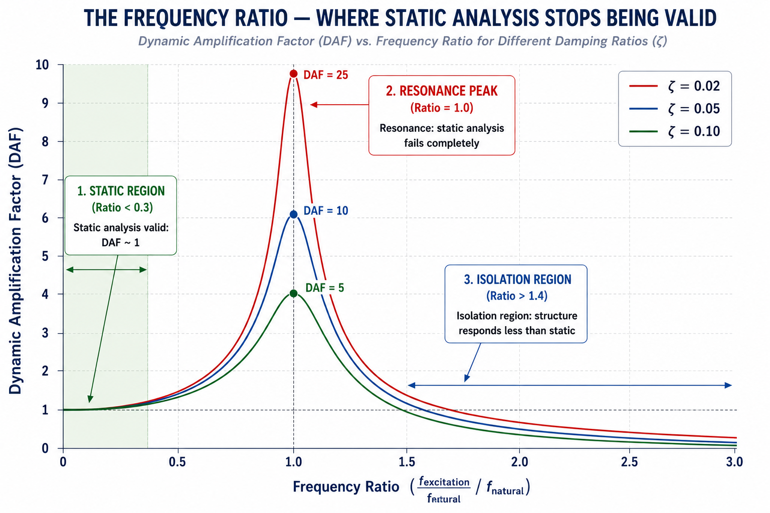
Static analysis is the special case where inertia forces (M·u”) and damping forces (C·u’) are both set to zero, reducing the equation to K·u = F. This is valid when the applied load changes so slowly that the structure has time to reach equilibrium at each instant, the velocity and acceleration are negligibly small compared to the displacement. The condition for this is that the frequency of load variation is much smaller than the structure’s natural frequency: specifically, the frequency ratio f_load / f_natural must be less than approximately 0.2 to 0.3 for the static result to be within 10 percent of the dynamic result.
Dynamic analysis retains the full equation of motion. The mass matrix M represents the inertia of the structure, its resistance to acceleration. The damping matrix C represents energy dissipation through material hysteresis, friction, fluid interaction, and other mechanisms. When the load changes rapidly or oscillates at a frequency near the structure’s natural frequencies, the inertia and damping terms are no longer negligible, they can dominate the response entirely, producing stresses orders of magnitude above or below what static analysis would predict.
The Mass Matrix: Where Dynamic Analysis Begins
Building a dynamic FEA model requires one critical input that static analysis does not need: mass distribution. The mass matrix M is assembled from element mass matrices, which are computed from the material density and element volume. An error in material density, a missing mass (non-structural mass not included in the element formulation), or a concentrated mass attachment not represented in the model will shift the natural frequencies away from their true values, potentially by 10 to 30 percent, changing the frequency ratios and making the dynamic analysis results unreliable.
The two approaches to mass matrix formulation are the consistent mass matrix (derived from the same shape functions as the stiffness matrix, producing a full matrix) and the lumped mass matrix (diagonal, with mass concentrated at nodes). Consistent mass matrices are more accurate for wave propagation and higher-mode response. Lumped mass matrices are computationally cheaper and are the default in explicit dynamics solvers because they allow direct computation of acceleration without a matrix solve. For modal analysis and harmonic response where lower modes dominate, both approaches give similar results for well-meshed models.
Damping: The Parameter Engineers Most Often Get Wrong
Damping determines how large the stress amplification is at resonance and how quickly the structure settles after an impulse. In FEA, damping is almost universally specified as Rayleigh damping: C = α·M + β·K, where α (mass-proportional) and β (stiffness-proportional) are constants calibrated from a target damping ratio at one or two natural frequencies. The damping ratio ζ (zeta) at a natural frequency ω_n is: ζ = α/(2ω_n) + βω_n/2.
Typical damping ratios for engineering structures: steel structures, 1 to 2 percent (0.01 to 0.02); reinforced concrete, 3 to 7 percent; soil and foundation systems, 10 to 20 percent; rubber mounts and elastomeric isolators, 5 to 15 percent. Using the wrong damping ratio has its greatest effect at resonance: at a frequency ratio of 1.0, the Dynamic Amplification Factor is 1/(2ζ). At 1 percent damping, DAF = 50. At 5 percent damping, DAF = 10. At 10 percent damping, DAF = 5. An error in damping ratio of a factor of two changes the resonance peak stress by a factor of two, a larger sensitivity than almost any other modeling parameter in structural FEA.
The Dynamic Amplification Factor: Quantifying When Static Analysis Fails
The Dynamic Amplification Factor (DAF) is the ratio of the maximum dynamic displacement (or stress) to the static displacement (or stress) that the same load magnitude would produce if applied statically. For a single-degree-of-freedom system under harmonic excitation:
DAF = 1 / √[(1 – r²)² + (2ζr)²]
where r = f_excitation / f_natural is the frequency ratio and ζ is the damping ratio. This formula is the single most important quantitative tool for deciding whether static analysis is sufficient:
- r < 0.3: DAF is between 1.0 and 1.10 for any realistic damping. Static analysis is valid, the dynamic correction is less than 10 percent, typically within the accuracy of the load specification itself.
- 0.3 < r < 0.7: DAF rises from 1.10 to between 1.5 and 2.5 depending on damping. Dynamic analysis is recommended. Static analysis underestimates peak stress by 50 to 150 percent in this range.
- 0.7 < r < 1.3 (resonance zone): DAF can reach 5 to 50 depending on damping. Static analysis is dangerously non-conservative. A structure with a safety factor of 3.0 from static analysis may have an effective safety factor below 1.0 if the frequency ratio is near 1.0.
- r > 1.4 (isolation region): DAF drops below 1.0, the dynamic response is actually less than the static response. Vibration isolators operate in this region deliberately. Static analysis is conservative (overestimates stress) but dynamic analysis gives a less conservative and more accurate result.
Worked Example: Frequency Ratio Check for a Pump Bracket
A steel pump bracket has a first natural frequency of 35 Hz (from a modal analysis or hand calculation using the bracket geometry and mass). The pump operates at 1,750 RPM, producing a vibration excitation at 1750/60 = 29.2 Hz. The pump also has a blade-passing frequency of 4 blades x 29.2 Hz = 116.7 Hz.
Frequency Ratio and DAF Calculation, Pump Bracket |
The Six Types of Dynamic Analysis: Which One to Use
Dynamic analysis is not a single method, it is a family of six distinct analysis types, each designed for a different class of dynamic loading. Choosing the wrong type is as consequential as choosing static analysis when dynamic is needed: a harmonic response analysis cannot capture the transient response to an impact, and a transient analysis is unnecessary and expensive when the excitation is steady-state sinusoidal. The following table maps each type to its use case, output, and solver approach.
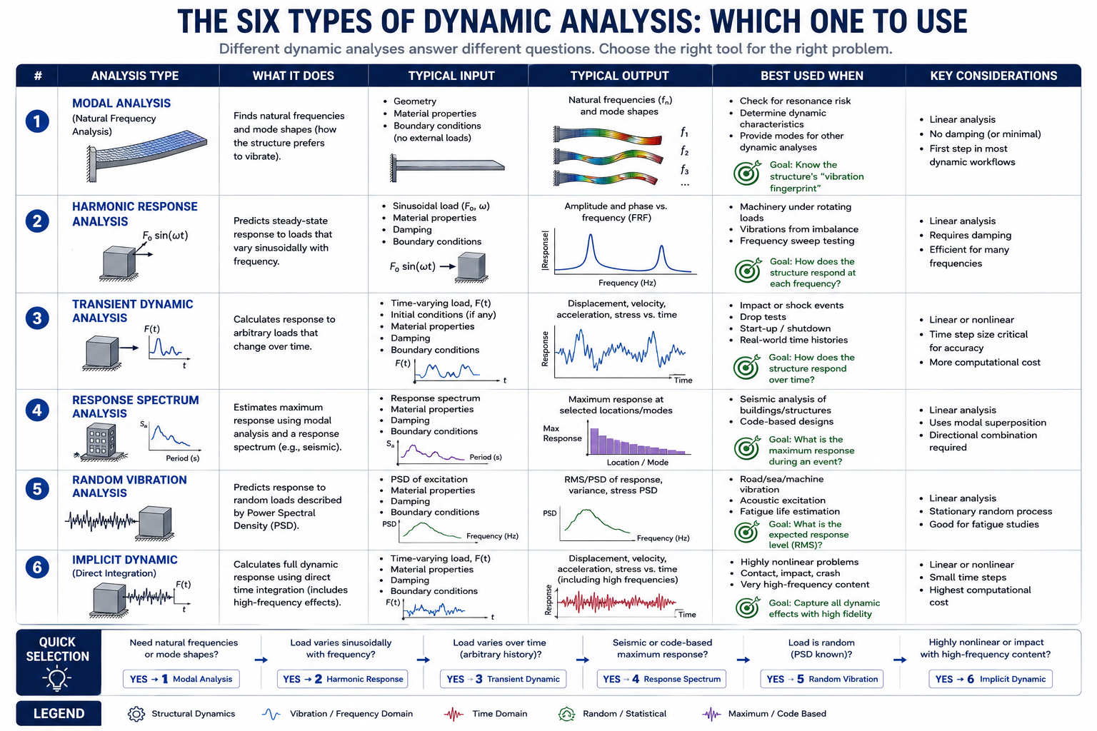
| Analysis Type | What It Solves | Primary Output | Typical Use Cases | Solver Approach |
| Modal / Natural Frequency | Undamped free-vibration: K·phi = omega^2·M·phi | Natural frequencies (Hz) and mode shapes | Finding resonant frequencies before designing excitation; validating FEA model against measured frequencies; selecting operating speeds for rotating machinery | Eigenvalue extraction (Lanczos, subspace iteration) |
| Harmonic Response (Frequency Response) | Steady-state response to sinusoidal excitation at each frequency | Amplitude and phase of displacement/stress vs frequency; frequency response functions (FRFs) | Rotating machinery vibration at operating speed and harmonics; acoustic noise excitation; vibration isolation design; modal testing correlation | Modal superposition across frequency sweep, or direct frequency response |
| Transient / Time History | Full time-domain response to arbitrary time-varying load F(t) | Displacement, velocity, acceleration, stress as functions of time | Impact and shock loads; seismic time history; drop tests; explosive events; any load that is not steady-state sinusoidal | Direct time integration (Newmark-beta, HHT-alpha) or modal superposition (more efficient for linear systems) |
| Response Spectrum | Statistical peak response to a spectrum of excitation (e.g., seismic design spectrum) | Peak displacements and stresses combined by modal combination rule (SRSS, CQC) | Seismic design of structures and equipment per building codes (ASCE 7, IBC, Eurocode 8); nuclear equipment qualification | Modal analysis + spectral acceleration read-off + modal combination |
| Random Vibration (PSD) | RMS response to broadband random excitation described by Power Spectral Density | RMS displacement, stress; PSD of response; fatigue damage spectrum | Aerospace launch environment qualification; road vehicle vibration; electronic PCB under random base excitation; MIL-STD-810 testing | Modal superposition + statistical integration over PSD input spectrum |
| Explicit Dynamics | Large deformation, short-duration, high-velocity transient with contact and material nonlinearity | Full time history of stress, strain, deformation including plastic flow, fracture, contact impact | Crash and impact simulation; blast and ballistic analysis; metal forming; bird strike; dropped object analysis | Explicit time integration (central difference); very small time steps (~microseconds) |
Modal Analysis: The Foundation of All Dynamic Analysis
Modal analysis, the computation of natural frequencies and mode shapes, is not just one type of dynamic analysis. It is the foundation on which harmonic response, response spectrum, and random vibration analyses are all built. Understanding modal analysis results is the prerequisite for interpreting every other dynamic output.
The natural frequencies ω_n (in rad/s) and mode shapes φ_n are the solutions to the eigenvalue problem: (K – ω_n²·M)φ_n = 0. Each mode shape φ_n describes the pattern of relative displacement across the structure when it vibrates at its corresponding natural frequency f_n = ω_n / (2π). The first (lowest) natural frequency is the most important: it defines the boundary between quasi-static and dynamic loading, and it is where the largest resonance amplification occurs for most realistic excitation spectra.
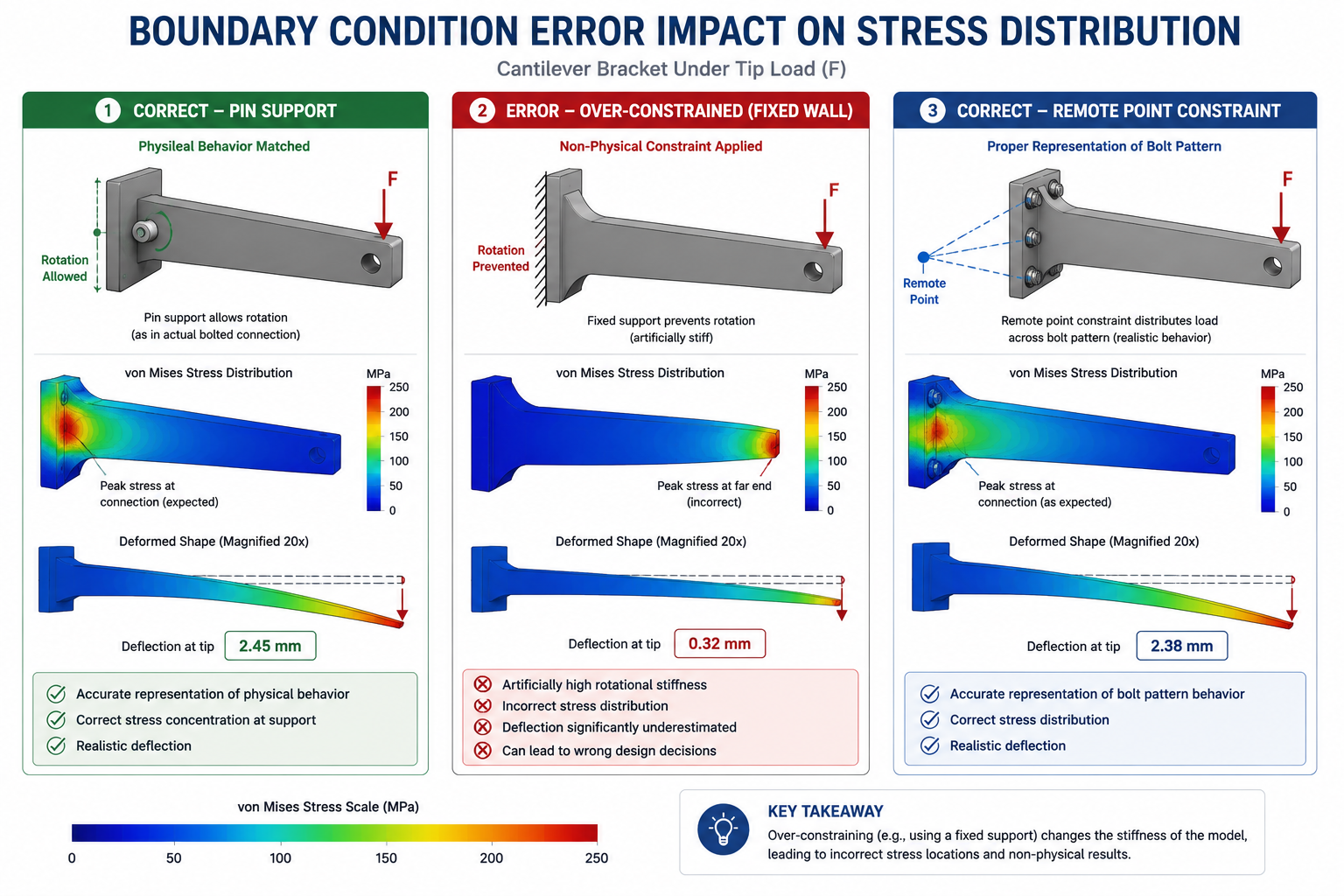
Read more on How to Select Boundary Conditions in FEA (With Examples)
Modal Effective Mass: Identifying Which Modes Matter
A structure with thousands of elements has thousands of natural frequencies and mode shapes. In practice, only a small number of modes contribute significantly to the response for any given loading direction. The modal effective mass for each mode and each direction tells the analyst what fraction of the total structural mass participates in that mode’s response to a base excitation in that direction. Modes with high effective mass dominate the response; modes with low effective mass can be neglected.
The standard criterion for modal truncation: include enough modes so that the cumulative effective mass exceeds 90 percent of the total structural mass in each excitation direction. For seismic analysis, ASCE 7 and Eurocode 8 require 90 percent mass participation. For general dynamic analysis, this criterion ensures that the missing higher modes contribute less than 10 percent to the total response, typically acceptable given other modeling uncertainties. Failing to include enough modes is the most common error in modal superposition analyses, producing results that appear converged but are missing significant response contributions from higher modes.
Interpreting Mode Shapes: What They Tell You About Failure Risk
Mode shapes tell the analyst where the structure is most flexible and where stresses will be highest if that mode is excited. A mode shape with large relative displacement at a specific location (a cantilevered arm tip, a thin web between flanges, a long unsupported span) indicates that if the excitation frequency is near this mode’s natural frequency, the stress at the high-displacement locations will be amplified by the DAF. Conversely, locations that show minimal motion in the mode shape are insensitive to excitation of that mode.
The practical application: after running a modal analysis, animate the first five to ten modes and identify which structural features participate in each. Then check whether any operational excitation frequencies (rotating machinery harmonics, flow-induced vibration, traffic loading rates) fall near any of these natural frequencies. This frequency map, plotting operational excitation frequencies against structural natural frequencies, is the single most useful deliverable from a modal analysis and the primary tool for identifying resonance risk before a component enters service.
Transient vs Harmonic Analysis: Choosing the Right Dynamic Solver
When dynamic analysis is required, the next decision is whether the loading is steady-state sinusoidal (harmonic) or time-varying and non-periodic (transient). This determines whether to use harmonic response analysis or transient time-history analysis, two fundamentally different solvers with different computational requirements, output formats, and appropriate post-processing approaches.
Harmonic Response Analysis
Harmonic response analysis solves for the steady-state amplitude and phase of structural response across a range of excitation frequencies. The input is a sinusoidal force or displacement excitation of specified amplitude, and the output is how the structure responds to that excitation at each frequency, the Frequency Response Function (FRF). The analysis sweeps through a user-defined frequency range, solving for the response at each frequency point.
Harmonic response is the correct tool for: rotating machinery at known operating speeds (where the imbalance force is sinusoidal at the rotation frequency and its harmonics), acoustic excitation (where the acoustic pressure is often a known sinusoidal signal), vibration test correlation (where shake-table tests apply sinusoidal excitation), and any application where the excitation is a steady, repetitive sinusoidal signal. It is not appropriate for impact, shock, seismic, or random vibration loading, all of which require transient or spectrum-based methods.
Transient (Time History) Analysis
Transient analysis solves the full equation of motion step by step through time, computing the displacement, velocity, acceleration, and stress at each time increment. The input is a complete time history of the applied load F(t). The output is the complete time history of structural response, how the structure evolves from its initial state through the loading event.
Two approaches to transient analysis: modal superposition transient (decompose the response into modal coordinates, solve each mode’s 1-DOF equation through time, then recombine, efficient for linear problems where the modes are computed once and the time integration is inexpensive) and direct time integration (solve the full system of equations at each time step using the Newmark-beta or HHT-alpha algorithm, more expensive but required for nonlinear problems where the stiffness or mass changes during the response, such as contact opening/closing or plasticity).
The critical time step selection rule for direct transient integration: the time step must be smaller than approximately T_n/20 for the highest mode of interest, where T_n is the natural period of that mode. For a structure with a highest significant natural frequency of 100 Hz (T = 10ms), the time step must be 0.5ms or smaller. Exceeding this limit produces numerical instability or artificial damping in the Newmark method, corrupting the high-frequency response.
| IMPLICIT vs EXPLICIT Time Integration: The Most Important Dynamic Solver Choice Implicit integration (Newmark-beta, HHT-alpha) solves a system of equations at each time step, stable for larger time steps but requires a matrix solve at every increment. Used for structural dynamics where the time step is governed by accuracy, not stability. Explicit integration (central difference) computes the next state directly from the current state without a matrix solve, extremely fast per step but conditionally stable: the time step must be smaller than the Courant stability limit (approximately element size / wave speed), typically microseconds for metal structures. Use implicit for structural vibration, seismic, and most transient problems. Use explicit only for very short-duration high-rate events (crash, blast, impact, metal forming) where the required time step is already in the microsecond range and the nonlinearity requires it. |
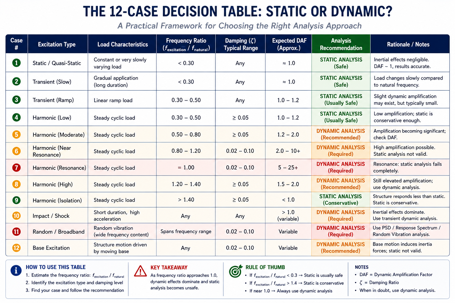
The 12-Case Decision Table: Static or Dynamic?
The following table maps 12 common engineering scenarios to the correct analysis type, with the rationale for each decision. Use this table as the starting point for any new analysis setup, identify the scenario closest to the problem at hand, check the rationale, and verify with the frequency ratio calculation before committing to a static or dynamic approach.
| Scenario | Load Characteristics | Recommended Analysis | Rationale |
| Lifting lug on a crane hook | Dead weight of lifted object; lift speed is slow | Static | Frequency ratio f_load/f_nat << 0.1; inertia forces negligible; DAF ~ 1.0 |
| Bridge under traffic loads | Vehicles crossing at known speeds; load varies slowly relative to bridge period | Static with dynamic amplification factor (code-specified) | Bridge codes (AASHTO, Eurocode) apply DAF to static result; full dynamic only for unusual load cases |
| Electric motor mounting bracket | Rotating imbalance force at motor RPM frequency | Harmonic response | Steady-state sinusoidal excitation at known frequency; must check if operating frequency is near natural frequency |
| Pump impeller under operating loads | Centrifugal load + blade-passing frequency excitation | Modal + harmonic response | Need natural frequencies to avoid resonance, then harmonic to quantify vibration at operating and blade-pass frequencies |
| Drop test of electronic enclosure | Impact with ground; very short duration (milliseconds) | Explicit dynamics or transient implicit | High-rate impulsive load; inertia forces dominate; duration comparable to or shorter than structural natural period |
| Seismic qualification of equipment | Earthquake ground motion, broadband, random-like | Response spectrum (code) or time history transient | Seismic codes specify response spectrum method; time history used when code spectrum is not applicable or for detailed assessment |
| PCB under launch vibration | Broadband random vibration, PSD specification (e.g., MIL-STD-1540) | Random vibration (PSD) | Excitation is statistical; RMS stress used for fatigue life prediction; deterministic transient is not meaningful for random inputs |
| Pressure vessel under static internal pressure | Constant internal pressure; no cyclic component | Static | Time-invariant load; structure not vibrating; linear static is exact solution |
| Heat exchanger tube under flow-induced vibration | Fluid cross-flow excites vortex shedding at Strouhal frequency | Modal + harmonic or transient | Must verify that vortex shedding frequency does not coincide with tube natural frequency; lock-in risk |
| Crankshaft torsional vibration | Engine firing pulses at multiples of RPM frequency | Modal + harmonic (torsional) | Torsional resonances can fracture crankshafts; must map all engine order excitations against torsional natural frequencies across RPM range |
| Blast-loaded wall panel | Explosive pressure pulse, millisecond duration | Explicit dynamics | Extreme strain rates; large deformation and possible fracture; implicit transient is too slow and may not handle the nonlinearity |
| Gravity-loaded shelf structure | Self-weight + uniformly distributed load; no vibration | Static | Classic static problem; any dynamic analysis would give identical result to static at zero cost premium |
Worked Examples: Static vs Dynamic Decision in Practice
Example 1: Overhead Crane Girder, Static Is Correct
An overhead crane girder spans 20 meters and carries a 10-tonne hoist. The crane travels at 0.5 m/s. Determine whether static or dynamic analysis is appropriate for the girder design check.
Natural frequency estimate: For a simply supported steel beam, f_1 = (π/2L²)√(EI/μ), where L = 20m, E = 210 GPa, I = moment of inertia of the girder section, μ = mass per unit length. For a typical crane girder with I = 0.004 m⁴ and mass 500 kg/m: f_1 ≈ 2.1 Hz.
Load frequency: The hoist travel at 0.5 m/s traverses the span in 40 seconds, corresponding to a loading frequency of approximately 1/40 = 0.025 Hz for the moving load cycle.
Frequency ratio: r = 0.025 / 2.1 = 0.012, far below 0.3. Static analysis is valid. Crane design codes (CMAA, FEM, Eurocode 3) specify dynamic load factors of 1.1 to 1.3 applied to the static load to account for the small dynamic amplification at this frequency ratio. Full dynamic analysis is not required and would produce essentially the same result as static with the code-specified dynamic factor applied.
Example 2: Compressor Skid Frame, Dynamic Analysis Required
A compressor skid frame supports a reciprocating compressor running at 750 RPM. The compressor produces primary and secondary unbalance forces at 12.5 Hz and 25 Hz respectively. A modal analysis of the skid frame shows natural frequencies at 18 Hz, 31 Hz, and 47 Hz.
Frequency ratios:
- Primary force (12.5 Hz) vs first mode (18 Hz): r = 12.5/18 = 0.694, approaching resonance zone. DAF at 2% damping: approximately 2.0
- Secondary force (25 Hz) vs second mode (31 Hz): r = 25/31 = 0.806, in resonance zone. DAF at 2% damping: approximately 3.6
- Secondary force (25 Hz) vs first mode (18 Hz): r = 25/18 = 1.39, just above resonance, DAF approximately 0.9
Decision: Harmonic response analysis is required for all operating speed combinations. The secondary force is within the resonance zone of the second skid mode, producing a DAF of 3.6. A static analysis using only the peak unbalance force magnitude would underpredict dynamic stress by a factor of 3.6 at this condition. The skid frame design must either be stiffened to shift natural frequencies away from operating harmonics, or damping must be added to reduce the DAF at the near-resonant condition.
Example 3: Equipment Seismic Qualification, Response Spectrum
An electrical cabinet weighing 800 kg must be qualified to the seismic requirements of IEEE 693 for moderate seismic risk. The facility is located in a region where the design seismic spectrum has a peak spectral acceleration of 0.5g at 5 Hz, falling to 0.2g at 20 Hz. The cabinet’s fundamental frequency from modal analysis is 8 Hz.
Decision: Response spectrum analysis is the correct method. The seismic excitation is broadband and statistical, a single time history is not representative of all possible earthquakes. The response spectrum provided by IEEE 693 (or the site-specific spectrum from a seismic hazard analysis) captures the statistical envelope of ground motion demands across all frequencies.
Procedure: Run modal analysis to find all modes with significant effective mass (target: 90% total mass participation in each direction). Read spectral acceleration from the design spectrum at each mode’s natural frequency. Compute peak modal response for each mode. Combine modal responses using SRSS (Square Root of Sum of Squares) or CQC (Complete Quadratic Combination) depending on frequency spacing. The resulting peak stress is used for structural qualification against code-allowable limits.
Key output: At 8 Hz, the spectral acceleration is approximately 0.45g (interpolated from the spectrum). The peak seismic inertia force on the cabinet is F = m·Sa = 800 kg × 0.45 × 9.81 m/s² = 3,532 N. This force is applied at the cabinet center of mass in the modal direction to determine base shear, anchor bolt loads, and internal component stress. A static analysis using only the code-specified static coefficient (0.2g in many older codes) would underestimate the dynamic demand at the 8 Hz frequency by a factor of 2.25.
When Static Analysis Masquerades as Sufficient
The most dangerous failure mode in analysis selection is not obvious error, it is static analysis that produces plausible results for the wrong reason. Several conditions make a static analysis appear adequate even when dynamic effects are significant:
The Safety Factor Absorbs the Dynamic Amplification, Until It Doesn’t
In many design codes and company standards, safety factors of 2.0 to 3.0 are applied to static stress results. If the dynamic amplification factor is 1.5 to 2.0, the safety factor may inadvertently cover the dynamic effect, and no fatigue cracking or yielding occurs during the design life. The analysis appears validated by the absence of field failures, but it is validated by coincidence, not by analysis correctness. When the operating speed changes, the excitation changes, the damping decreases due to wear, or a slightly different component with a different natural frequency is installed, the coincidental coverage disappears and failures begin.
Operating Below Resonance, And Then Crossing Through It
A machine that operates below its resonance frequency (r < 0.7, DAF < 1.5) during normal operation passes through resonance every time it starts up or shuts down. If the run-up time is short (seconds), the structure spends little time at resonance and the peak transient amplification is limited. If the run-up time is long (minutes), the structure can build up resonance amplitude over many cycles, a phenomenon called resonance dwell that can produce stresses far exceeding the steady-state resonance peak. Machines with long coast-down times under power failure are particularly vulnerable: the speed decays slowly through the resonance zone while the structure vibrates at peak amplitude.
Low-Damping Materials at Near-Resonant Conditions
Steel and aluminum structures have inherently low material damping (0.5 to 2 percent critical damping). At frequency ratios between 0.8 and 1.2, the DAF for 1 percent damping ranges from 5 to 50. A static analysis that ignores this amplification is not conservative by a factor of 2, it is non-conservative by a factor of 5 to 50. Any steel or aluminum structure with a known excitation source at a frequency within 30 percent of any natural frequency requires dynamic analysis, regardless of the apparent static safety factor.
Frequently Asked Questions
Q: What is the frequency ratio and how do I use it to decide between static and dynamic analysis?
The frequency ratio r = f_excitation / f_natural is the ratio of the load’s frequency of variation to the structure’s first natural frequency. When r is less than 0.3, the Dynamic Amplification Factor (DAF) is within 10 percent of 1.0 for any realistic damping, and static analysis is valid. When r is between 0.3 and 0.7, the DAF rises to between 1.1 and 2.5, and dynamic analysis is recommended. When r approaches 1.0 (resonance), the DAF can reach 5 to 50 depending on damping, and static analysis is completely invalid, it underestimates peak stress by factors of 5 to 50.
To use the frequency ratio: (1) estimate or measure the structure’s first natural frequency by modal analysis or hand calculation, (2) identify all significant excitation frequencies (RPM harmonics, vortex shedding, flow pulse rates, etc.), (3) compute r for each excitation/mode pair, and (4) apply the DAF formula to quantify the amplification. If DAF exceeds 1.1 for any significant excitation, dynamic analysis is required.
Q: What is the difference between modal analysis and dynamic analysis?
Modal analysis is one specific type of dynamic analysis that computes the natural frequencies and mode shapes of a structure by solving the eigenvalue problem (K – omega^2 * M) * phi = 0. It does not compute response to any applied load, it only characterizes the free-vibration properties of the structure. Dynamic analysis is a broader term covering all analysis types that include inertia effects: modal analysis, harmonic response, transient time history, response spectrum, random vibration (PSD), and explicit dynamics. Modal analysis is typically the first step in a complete dynamic analysis workflow: run modal to find natural frequencies and mode shapes, then use those results as the basis for harmonic, response spectrum, or random vibration analyses using modal superposition.
Q: Can I use a Dynamic Amplification Factor with a static analysis instead of running a full dynamic analysis?
Yes, for many standard applications, this is exactly what building codes (ASCE 7), crane codes (CMAA, Eurocode 3), and seismic codes do when they specify a dynamic load factor or dynamic amplification factor to be applied to a static load. The approach is valid when: (1) the excitation frequency and the dominant natural frequency are both known, (2) the frequency ratio places the system in a predictable DAF region (not in the chaotic high-sensitivity zone near resonance), and (3) the code-specified DAF conservatively bounds the actual dynamic amplification for the load case.
When the frequency ratio is near 1.0, code-specified DAFs are no longer reliable bounds and a full dynamic analysis is required to determine the actual amplification. Also note that DAF-amplified static analysis cannot predict resonance, mode shape effects on stress distribution, or transient build-up phenomena, it only adjusts the magnitude of the static load.
Q: What is explicit dynamics and when does it replace implicit transient analysis?
Explicit dynamics uses the central difference time integration method to step forward in time without solving a system of equations at each step, each node’s acceleration is computed directly from the forces on it, then integrated to velocity and displacement. This makes each time step very fast computationally, but the method is only conditionally stable: the time step must be smaller than the Courant stability limit, typically the element size divided by the acoustic wave speed in the material (microseconds for steel).
Q: Why does my static FEA agree with my hand calculation but my test shows three times higher stress?
This is the signature of an unidentified dynamic effect. When static FEA and analytical statics agree but physical testing shows much higher stress, the most likely cause is that the test excitation frequency is near a natural frequency of the structure, producing resonance amplification that neither the static FEA nor the hand calculation can capture.
Q: How many modes do I need to include in a modal superposition analysis?
Include enough modes so that the cumulative modal effective mass exceeds 90 percent of the total structural mass in each excitation direction. This is the minimum requirement specified by seismic codes (ASCE 7, Eurocode 8) and is a reasonable criterion for general dynamic analysis. In practice, this typically requires 10 to 50 modes for typical industrial structures, more for complex structures with distributed mass.
Conclusion:
Static analysis is not a simplification of dynamic analysis. It is a different answer to a different question. Static analysis asks what the stress is under a constant, equilibrium load. Dynamic analysis asks what the stress is when the load varies with time and when the structure’s inertia and natural frequencies determine how it responds. For slowly applied loads far below the first natural frequency, these questions have the same answer. For any other loading condition, they diverge, and the divergence grows without bound as the excitation frequency approaches the structural resonance.
The decision process is: calculate the frequency ratio, evaluate the DAF, and let the physics determine the analysis type. Not the software default, not the schedule pressure, not the analyst’s familiarity with static setups. A structure with a known excitation at 80 percent of its first natural frequency has a minimum DAF of 2.8 at 2 percent damping, the static safety factor must exceed 2.8 just to break even with the dynamic effect, before any structural uncertainty is accounted for. No engineering practice justifies static analysis in that condition.
The tools for making the correct decision are in this article: the governing equation that shows exactly which terms static analysis drops, the DAF formula that quantifies the error of ignoring them, the six dynamic analysis types and their appropriate load cases, the 12-case decision table, and the worked examples showing the calculation chain from operating RPM to frequency ratio to DAF to required analysis type. Apply this framework at the beginning of every analysis setup, before any model is built.
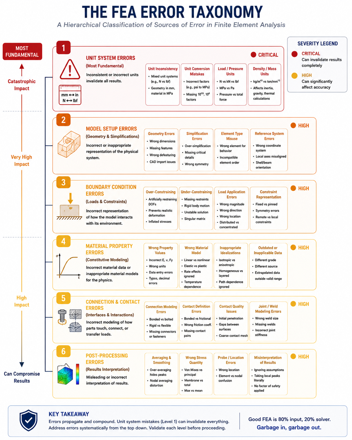
Continue your FEA knowledge with our guides on boundary condition selection, stress concentration analysis, mesh quality and convergence, linear vs nonlinear FEA, and common FEA errors that produce wrong results.