The 40-millimeter-diameter shaft that the engineer specified should have been more than adequate for the applied torque. The calculation showed it. But the shaft failed in fatigue after three months of service, and the failure initiated at the shoulder fillet where the shaft stepped down to its smaller diameter. The shoulder fillet radius was 0.5 millimeters. The torque was well within the material’s endurance limit. The stress concentration at that 0.5mm radius was not.
This is the pattern of stress concentration failure: an engineer calculates a safety factor using the nominal stress at the critical section, the factor looks adequate, and the component fails because the local peak stress at the geometric discontinuity was never considered. The nominal stress is the average stress across the net cross-section. The actual peak stress at a notch, hole, fillet, or groove is a multiple of that nominal: for a small-radius fillet on a large shoulder, that multiple can exceed 3 or 4, consuming the entire safety factor and putting the local stress into the fatigue damage regime even when the nominal stress calculation suggests otherwise.
Stress concentration analysis is the engineering discipline of quantifying this peak-to-nominal stress ratio, understanding what governs it, and designing to control it. This article covers the complete framework: the physics of stress concentration, the mathematical definitions of the theoretical stress concentration factor Kt and the fatigue notch factor Kf, practical Kt values for 14 common engineering geometries, the notch sensitivity factor that connects Kt to Kf for real materials, the step-by-step workflow for extracting Kt from FEA, and the design strategies that reduce stress concentrations at the CAD stage before they become fatigue problems in service.
The Physics of Stress Concentration: Why Geometry Creates Local Peaks
Stress concentration is not a failure of the stress calculation: it is a physical reality of how elastic bodies transmit force through geometric discontinuities. To understand it intuitively, think of stress lines as analogous to streamlines in a fluid flow. When fluid flows through a uniform pipe, the streamlines are evenly distributed across the cross-section. When the pipe has a constriction, the streamlines must crowd together at the narrowest point. The velocity at the constriction is higher than in the uniform pipe: the same flow rate must pass through a smaller area.
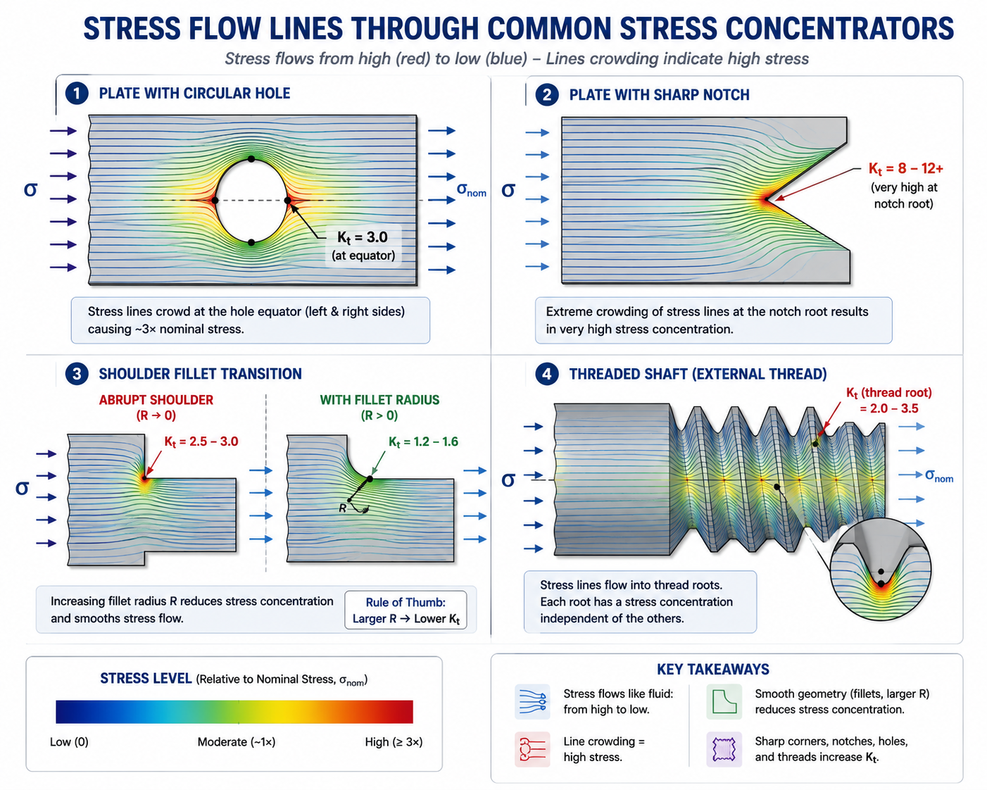
Stress transmission in an elastic solid follows the same principle. Under uniform tensile loading, the stress is uniformly distributed across a uniform cross-section. At a geometric discontinuity, the stress lines must redirect around the discontinuity and then reconverge. The stress lines crowd together at the most constrained point of the discontinuity, producing a local peak that is higher than the average stress in the net cross-section. The ratio of this local peak to the average is the stress concentration factor Kt.
The Circular Hole in a Plate: The Exact Solution
The most important exact solution in stress concentration analysis is the Kirsch solution for an infinite plate with a circular hole under uniaxial tension. Derived by Ernst Kirsch in 1898, this solution gives the complete stress field around the hole in closed form. At the edge of the hole on the axis perpendicular to the applied load (the equator of the hole), the stress in the loading direction is exactly three times the remote stress. At the edge of the hole on the axis parallel to the load (the poles of the hole), the stress in the loading direction is compressive and equal to minus one times the remote stress (full stress reversal).
This Kt = 3 for a circular hole in an infinite plate is perhaps the single most important number in mechanical engineering fatigue design. It appears in Peterson’s Stress Concentration Factors, in every textbook on machine design, and in every FEA validation exercise for stress concentration analysis. It is exact for an infinite plate (one where the hole diameter is negligibly small compared to the plate width). As the hole diameter approaches the plate width, the finite-width correction increases Kt above 3, eventually approaching infinity as the hole fills the plate.
The Kirsch solution also shows that stress concentration is a local phenomenon: the stress elevation decays rapidly with distance from the hole. At a distance equal to one hole radius from the edge of the hole (two hole radii from the center), the stress has already returned to within 10 percent of the remote stress. This decay behavior is the basis of Saint-Venant’s principle as applied to stress concentration: the elevated stress is confined to a region approximately equal to the size of the discontinuity, and the rest of the structure is essentially unaffected by the local stress elevation.
The Elliptical Hole: How Shape Controls Kt
The exact solution for an elliptical hole in an infinite plate under uniaxial tension gives Kt = 1 + 2(a/b), where a is the semi-axis perpendicular to the applied load and b is the semi-axis parallel to the applied load. For a circular hole (a = b), this gives Kt = 1 + 2(1) = 3, recovering the Kirsch result. For an ellipse elongated perpendicular to the load (a > b, a crack-like geometry), Kt grows without bound as a/b increases. For an ellipse elongated parallel to the load (a < b, a stream-lined hole), Kt decreases below 3, approaching 1 for a very elongated ellipse aligned with the load direction.
This formula contains the entire design principle of stress concentration reduction in one equation: the ratio of the semi-axis perpendicular to the load to the semi-axis parallel to the load determines Kt. To minimize Kt for a hole in a plate under uniaxial tension, orient the hole’s long axis parallel to the loading direction. This principle explains why aircraft fuselage windows are rounded-rectangle shapes (to reduce the Kt at the corners), why keyways are given generous corner radii (to reduce the b/a ratio at the key corner), and why sharp notches and cracks are so damaging (their extreme a/b ratio produces very high Kt values).
The Theoretical Stress Concentration Factor Kt: Definition and Reference Data
The theoretical stress concentration factor Kt is defined as the ratio of the maximum local stress at a geometric discontinuity to the nominal stress at the net cross-section:
Kt = sigma_max / sigma_nom
where sigma_max is the maximum stress at the discontinuity (from elastic analysis) and sigma_nom is the nominal stress calculated at the net cross-section using standard mechanics formulas (P/A for tension, Mc/I for bending, Tc/J for torsion). The subscript t in Kt indicates theoretical: this is the ratio from linear elastic theory, which overestimates the actual fatigue stress concentration factor in ductile materials because it does not account for the material’s ability to redistribute stress locally through microplasticity. The conversion from Kt to the fatigue-relevant factor Kf requires the notch sensitivity factor, covered in the next section.
Kt Reference Values for 14 Common Geometries
| Geometry | Loading | Kt Range | Key Parameter | Notes |
| Circular hole in infinite plate | Uniaxial tension | 3.0 (exact) | d/W -> 0 (infinite plate limit) | Kt=3 is exact for infinite plate; reduces with finite width |
| Circular hole in finite-width plate | Uniaxial tension | 3.0 to 10+ | d/W ratio (hole dia/plate width) | Kt increases sharply as d/W exceeds 0.5 |
| Elliptical hole in plate | Uniaxial tension | 1 + 2(a/b) | a/b (semi-axis ratio) | a=major axis perpendicular to load; Kt=3 for circle (a=b) |
| Shoulder fillet (rectangular bar) | Axial tension | 1.2 to 3.0 | r/d and D/d ratios | r=fillet radius, d=small width, D=large width |
| Shoulder fillet (rectangular bar) | Bending | 1.2 to 2.5 | r/d and D/d ratios | Lower Kt than tension for same geometry |
| Shoulder fillet (circular shaft) | Axial tension | 1.2 to 3.0 | r/d and D/d ratios | Similar to rectangular bar in tension |
| Shoulder fillet (circular shaft) | Bending | 1.2 to 2.5 | r/d and D/d ratios | Lower Kt than tension; use Pilkey/Peterson for exact values |
| Shoulder fillet (circular shaft) | Torsion | 1.1 to 2.0 | r/d and D/d ratios | Torsion Kt always lower than bending or tension Kt |
| Circumferential U-groove (shaft) | Bending | 1.5 to 4.0 | r/d (groove radius/shaft dia) | Sharper groove = higher Kt; deep groove compounds effect |
| Transverse hole in round shaft | Bending | 2.0 to 4.0 | d_hole/D_shaft | Very sensitive to hole diameter ratio |
| Keyway (sled runner type) | Torsion | 2.0 to 3.0 | r/b (corner radius/width) | Sharp keyway corners: Kt up to 5+; add corner radii |
| Metric thread (M-series) | Axial tension | 2.0 to 4.0 | Thread pitch and root radius | Root radius r = 0.144P for M-thread; Kt from thread profile charts |
| Press-fit interface (shaft/hub) | Bending | 1.5 to 3.0 | Press fit pressure, contact length | Fretting fatigue risk; Kt highly variable with fit tolerance |
| T-head bolt under bearing load | Bending + tension | 2.5 to 5.0 | Head geometry, fillet radius | Complex stress state; FEA recommended for accuracy |
Using Peterson’s Charts: What They Are and How to Read Them
The definitive reference for Kt in engineering practice is Peterson’s Stress Concentration Factors, originally published by R.E. Peterson and now in its fourth edition edited by Walter Pilkey and Deborah Pilkey (Wiley, 2020). Peterson’s charts provide Kt as a function of relevant geometric ratios for hundreds of configurations: plates with holes, shoulders and fillets, grooves and notches, keyways, threads, welds, and many other geometries that arise in mechanical design.
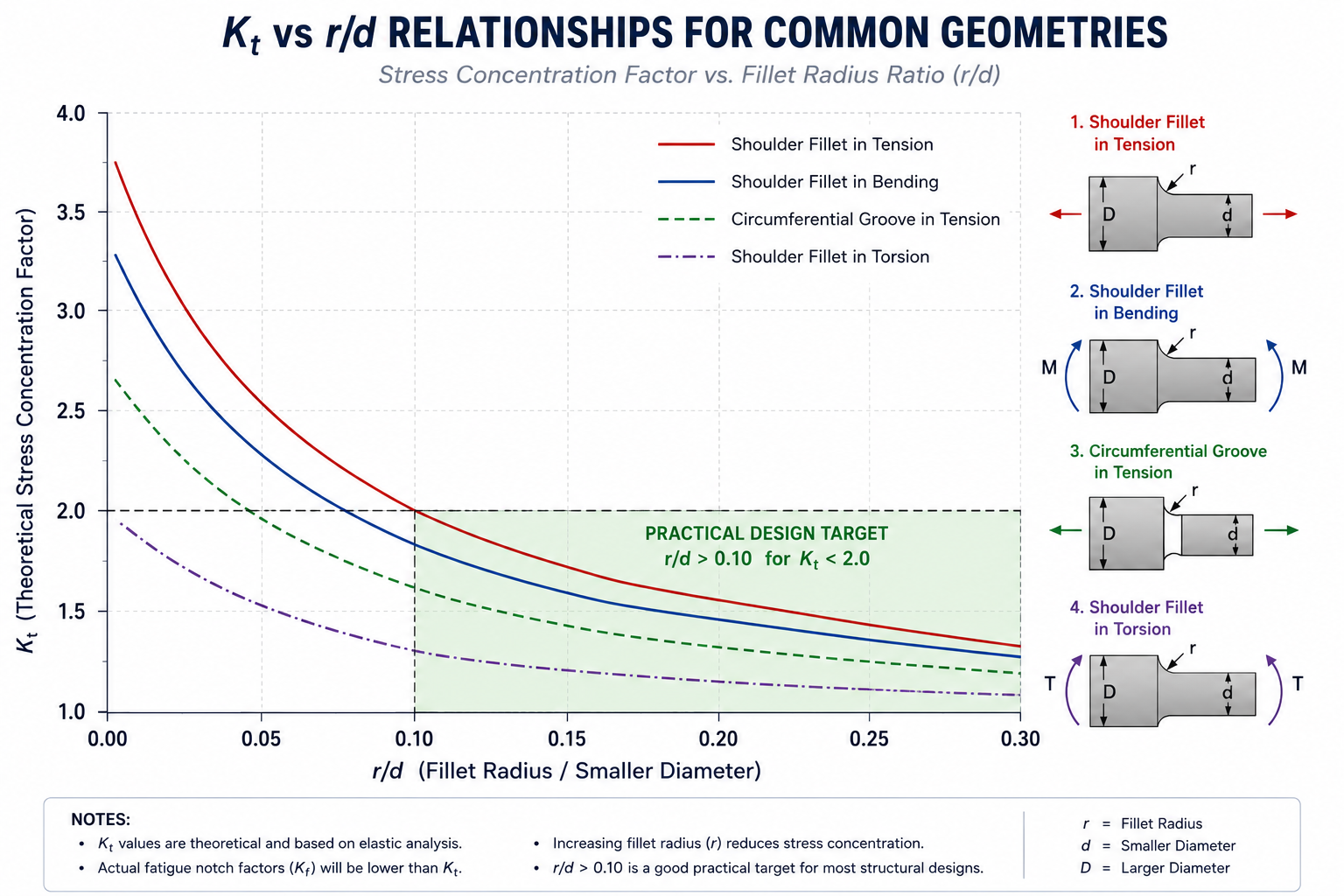
Each Peterson’s chart plots Kt on the vertical axis against one geometric ratio (typically r/d, where r is the root radius and d is the smaller cross-sectional dimension) with multiple curves for different values of a second geometric ratio (typically D/d for shoulder fillets, where D is the larger dimension). To use the chart for a specific geometry, determine the relevant geometric ratios from the dimensions, locate the appropriate curve, and read off the Kt value. Always verify that your geometric ratios fall within the validity range of the chart: the Pilkey edition explicitly states validity ranges, and extrapolating beyond them can introduce errors of 20 percent or more.
From Kt to Kf: Notch Sensitivity and the Fatigue Stress Concentration Factor
The theoretical stress concentration factor Kt is a geometric property. It depends only on the shape of the discontinuity, not on the material. Two components of identical geometry, one made of hardened steel and one made of rubber, have the same Kt. But they will behave very differently under cyclic loading, because the hardened steel is highly sensitive to the local peak stress while the rubber can redistribute that stress through local deformation without initiating fatigue damage.
The material’s sensitivity to stress concentrations in fatigue is captured by the notch sensitivity factor q, which ranges from 0 (completely insensitive to notches) to 1 (fully sensitive, experiencing the full theoretical stress concentration). The fatigue notch factor Kf is related to Kt and q by:
Kf = 1 + q(Kt – 1)
When q = 0: Kf = 1 (no effect of stress concentration on fatigue). When q = 1: Kf = Kt (full theoretical concentration applies). For most engineering materials, q lies between these extremes and depends on the material’s ultimate tensile strength, the notch root radius, and the notch geometry. Higher-strength materials have higher notch sensitivity: a hardened tool steel near its endurance limit will experience close to the full Kt effect at a notch, while a mild steel will experience perhaps 80 percent of Kt at the same notch geometry.
The Neuber Constant and Notch Sensitivity Calculation
The quantitative relationship between notch root radius r and notch sensitivity q is given by the Neuber equation
q = 1 / (1 + sqrt(a/r))
where r is the notch root radius in millimeters and a is the Neuber constant, a material property with units of length that characterizes the material’s sensitivity to stress gradients. The Neuber constant is determined from fatigue test data comparing notched and unnotched specimens. For common engineering materials:
| Material / Condition | Neuber Constant ‘a’ (mm) | Notch Sensitivity q at r=1mm | Notch Sensitivity q at r=5mm | Practical Implication |
| Annealed or normalized steel (Sut ~400-600 MPa) | 0.25 | 0.80 | 0.95 | High notch sensitivity; design with generous fillets |
| Quenched & tempered steel (Sut ~700-1000 MPa) | 0.064 | 0.94 | 0.99 | Very high sensitivity; Kf approaches Kt; fillet radius critical |
| High-strength steel (Sut >1000 MPa) | 0.025 | 0.98 | 1.00 | Essentially full notch sensitivity; Kf = Kt; stress concentration dominates fatigue |
| Aluminum alloys (Sut ~200-500 MPa) | 0.50 | 0.67 | 0.91 | Moderate sensitivity; less critical than high-strength steel |
| Cast iron (gray) | 2.5 | 0.29 | 0.67 | Low sensitivity; inherent porosity already acts as stress concentrator |
| Mild steel (annealed, Sut ~400 MPa) | 0.25 | 0.80 | 0.95 | Common structural steel; notch sensitivity substantial |
| Titanium alloys (Sut ~800-1200 MPa) | 0.10-0.25 | 0.85-0.95 | 0.97-0.99 | High sensitivity similar to Q&T steel; fatigue critical |
Worked Example: Calculating Kf for a Shoulder Fillet
A quenched and tempered steel shaft (Sut = 800 MPa) has a shoulder fillet with r = 2mm, small diameter d = 30mm, large diameter D = 40mm. The shaft is subject to bending. Determine Kf.
- Find Kt from geometry: r/d = 2/30 = 0.067; D/d = 40/30 = 1.33. From Peterson’s chart for shoulder fillet in bending: Kt approximately 1.85
- Find Neuber constant for Q&T steel at Sut = 800 MPa: a = 0.064 mm (from table above or Shigley’s/Peterson’s chart for a vs Sut)
- Calculate notch sensitivity: q = 1 / (1 + sqrt(0.064/2)) = 1 / (1 + sqrt(0.032)) = 1 / (1 + 0.179) = 1 / 1.179 = 0.848
- Calculate Kf: Kf = 1 + q(Kt-1) = 1 + 0.848(1.85-1) = 1 + 0.848 x 0.85 = 1 + 0.721 = 1.72
The fatigue notch factor Kf = 1.72 is the factor to apply to the nominal bending stress when computing the fatigue safety factor or performing a stress-life (S-N) analysis. The nominal endurance limit of the material is divided by Kf (and other fatigue modifying factors) to give the component endurance limit at this location. Using Kt = 1.85 instead of Kf = 1.72 would give a more conservative result (about 8% additional conservatism), which is acceptable and is the safer choice when q is uncertain
Extracting Kt From FEA: The Workflow That Bypasses Peterson’s Charts
For complex geometries where no Peterson’s chart exists, or where the geometry falls outside the validity range of existing charts, FEA provides a direct method for computing Kt. A converged elastic FEA model of a notched geometry directly computes Kt as the ratio of the peak stress to the nominal stress, without requiring any chart lookup or geometric approximation. The accuracy of the FEA-derived Kt depends entirely on the mesh quality at the notch root, as described in the mesh quality article in this series.
The FEA-Based Kt Extraction Protocol
- Build the geometry with the notch explicitly modeled: Do not approximate the fillet or notch geometry. The actual radius must be correctly represented in the CAD model. Errors in fillet radius of even 20 percent can change Kt by 10 to 20 percent.
- Apply linear elastic material: Kt is defined for elastic behavior only. Use a linear elastic material model. Do not apply plasticity at this stage.
- Apply consistent loading and boundary conditions: The nominal stress sigma_nom must be clearly defined. For tension Kt, apply a uniform remote stress and measure the nominal stress at the net cross-section (P/A). For bending Kt, apply a moment and measure the nominal bending stress at the net cross-section (Mc/I).
- Achieve mesh convergence at the notch root: The stress peak at the notch root is a steep gradient region. Run a mesh convergence study specifically at the notch root, refining the mesh until the peak stress changes by less than 2 percent between successive refinements. The first mesh level should have at least 4 to 6 elements spanning the fillet radius circumferentially. Convergence often requires 10 to 20 elements spanning the radius.
- Extract sigma_max from unaveraged nodal stress: At the converged mesh, extract the maximum principal stress (not von Mises) at the notch root using unaveraged nodal values. Von Mises stress averages the effect of multiple stress components; for Kt in uniaxial loading, the maximum principal stress at the loaded surface is the correct quantity.
- Calculate Kt: Kt = sigma_max / sigma_nom. The sigma_nom is the stress from the standard mechanics formula at the net section, computed independently of FEA (P/A, Mc/I, Tc/J as applicable). Do not use the FEA-predicted stress far from the notch as sigma_nom: use the analytical nominal stress formula.
- Verify against Peterson’s chart if available: For standard geometries (circular hole, shoulder fillet, U-notch), compare the FEA-derived Kt against the Peterson’s chart value for the same geometric ratios. Agreement within 5 percent confirms that the FEA mesh and extraction method are correct.
Peterson’s Stress
FEA Kt Extraction: Worked Numerical Example |
Stress Concentration in Fatigue Design: Applying Kf to Endurance Limit Calculations
In fatigue design, Kf appears as a modifier to the material’s nominal endurance limit. The modified endurance limit Se for a component at a specific notch location is:
Se = ka x kb x kc x kd x ke x (Se’ / Kf)
where Se’ is the material’s rotating-beam endurance limit (approximately 0.5 Sut for steels up to Sut = 1400 MPa, with decreasing ratio above this), ka is the surface finish factor, kb is the size factor, kc is the reliability factor, kd is the temperature factor, ke is any additional modifying factor, and Kf appears in the denominator as a strength reduction factor at the notch location
The Three Locations That Govern Fatigue Life in Shafts
In rotating shaft design, experience and research consistently identify three locations that most commonly initiate fatigue cracks: shoulder fillets, keyways, and press-fit interfaces. Understanding the Kf at each location determines which governs the fatigue design and where the analyst should focus geometry optimization.
A typical step-down shaft under combined bending and torsion will have the highest Kf at the shoulder fillet if the fillet radius is small (r/d < 0.05), at the keyway corner if the keyway has sharp corners (Kf up to 3.0 to 4.0 for sled-runner keyways), or at the press-fit edge if a gear or bearing hub is pressed onto the shaft (Kf from fretting fatigue effects). The engineer must calculate Kf at each of these three locations and design the fillet radii, keyway geometry, and press-fit stresses to keep the most critical Kf within the fatigue design target
Stress Concentration in Thread Connections
Threads represent a particularly important and often underestimated source of stress concentration. The thread root is a circumferential notch with a root radius determined by the thread standard: for standard metric M-threads, the root radius is approximately r = 0.144P, where P is the thread pitch. For an M8x1.25 bolt, the root radius is approximately 0.144 x 1.25 = 0.18mm. This very small radius, combined with the large step ratio at the thread root geometry, produces Kt values of 2.0 to 4.0 for threaded connections in tension
The location of highest stress in a bolt connection is almost always at the first engaged thread in the nut or tapped hole, where the applied tension load is highest and the thread-to-thread load distribution concentrates approximately 40 percent of the total load in the first thread. Combined with the thread root Kt, this makes the first-thread root the fatigue-critical location in virtually every bolt connection. Thread run-out, where the thread terminates at the shank, is the second critical location.
Reducing Stress Concentrations: Design Strategies at the CAD Stage
Stress concentrations are a design problem that is best solved at the CAD modeling stage, before geometry is committed to tooling. The following strategies reduce Kt and Kf at specific geometric features, with specific design guidelines that can be applied directly in the CAD environment.
Increasing Fillet Radii: The Most Effective and Simplest Strategy
The most direct way to reduce Kt at a shoulder fillet is to increase the fillet radius. The relationship between r/d and Kt is highly nonlinear: increasing r/d from 0.02 to 0.10 (a 5x increase in fillet radius) typically reduces Kt by 30 to 50 percent. Increasing r/d from 0.10 to 0.20 gives a further reduction of 10 to 20 percent. The largest proportional gains come from escaping the very small radius region (r/d < 0.05) where Kt rises sharply as the radius approaches zero.
The practical design target: r/d >= 0.10 for Kt below 2.0 for most shoulder fillet geometries. Where the design space allows, targeting r/d >= 0.20 achieves Kt below 1.5 for most fillet configurations. This corresponds to a fatigue life improvement of roughly 2 to 4 times compared to a tight fillet at r/d = 0.02 in high-strength steel, which has near-full notch sensitivity.
The Multiple Radius and Undercutting Approach
When the step in a shaft cannot accommodate a large fillet radius (because the shoulder face must be perpendicular and the transition distance is limited), two alternative geometric strategies reduce Kt without requiring a larger transition zone: multiple radius fillets and undercut grooves
A multiple radius fillet (sometimes called a compound fillet or Gough-Bell fillet) uses two or more radii blending together to transition from the small to the large shaft diameter. The smaller radius blends the geometry near the shoulder face, and the larger radius transitions the remaining step. The compound fillet achieves lower Kt than either radius alone because the stress flow lines are more gently redirected. The design is slightly more complex to machine but is standard practice in high-cycle fatigue applications such as crankshafts and turbine shafts.
An undercut groove (relief groove) is a small circumferential groove cut adjacent to the shoulder, parallel to the axis. This moves the stress concentration away from the shoulder face (where the contact stress from the bearing or hub adds to the bending stress) and provides a relief path for the stress flow. The undercut Kt is typically 10 to 20 percent lower than the equivalent shoulder fillet Kt and can be cut to a larger radius than the shoulder fillet because it is not constrained by the step height.
Drilling Adjacent Relief Holes for Keyways
The keyway corner is one of the most stress-concentrated regions in shaft design, with Kf values up to 3.0 to 5.0 for sharp sled-runner keyways. A particularly effective and practical reduction strategy is to drill small relief holes at the ends of the keyway, at the locations where the stress concentration is highest. The relief holes remove material exactly where the stress is highest, which seems counterintuitive, but the holes replace a sharp 90-degree internal corner with a smooth circular arc, which has dramatically lower Kt than the sharp corner.
Peterson’s data for keyways with end relief holes shows Kt reductions of 30 to 50 percent compared to sled-runner keyways without relief. The relief hole diameter is typically 0.5 to 1.0 times the keyway width. This approach is standard in power transmission shaft design for high-cycle applications.
Frequently Asked Questions
Q: What is a stress concentration factor (Kt)?
The stress concentration factor Kt is the ratio of the maximum local stress at a geometric discontinuity (hole, notch, fillet, groove) to the nominal stress at the net cross-section calculated by standard mechanics formulas (P/A for tension, Mc/I for bending, Tc/J for torsion). Kt is a dimensionless geometric factor that depends only on the shape of the discontinuity, not on the material or the load magnitude. For a circular hole in an infinite plate under uniaxial tension, Kt = 3 exactly (Kirsch solution). For sharp notches, Kt can exceed 5 to 10. Kt is used in fatigue analysis by converting it to the fatigue notch factor Kf through the notch sensitivity factor.
Q: What is the difference between Kt and Kf?
Kt (theoretical stress concentration factor) is purely geometric: it is the ratio of peak to nominal stress from linear elastic theory and depends only on the geometry of the notch. Kf (fatigue notch factor) is the ratio that actually reduces the fatigue endurance limit in practice. It accounts for the fact that ductile materials can partially redistribute stress at notch roots through microplasticity, reducing the effective stress concentration below the theoretical maximum. Kf is related to Kt by Kf = 1 + q(Kt-1), where q is the notch sensitivity factor (0 for no sensitivity, 1 for full sensitivity). For high-strength steels, q approaches 1 and Kf approaches Kt. For cast iron, q is close to 0 and Kf approaches 1.
Q: How do I find the stress concentration factor for a fillet or notch?
For standard geometries (shoulder fillets, circular holes, U-notches, keyways, threads), look up Kt in Peterson’s Stress Concentration Factors (Pilkey and Pilkey, Wiley) using the relevant geometric ratios: r/d (fillet radius to smaller dimension), D/d (larger to smaller dimension), d/W (hole diameter to plate width). For complex or non-standard geometries, build a converged linear elastic FEA model, apply the appropriate loading, extract the peak maximum principal stress at the notch root from unaveraged nodal values, and calculate Kt = sigma_max / sigma_nom where sigma_nom is computed from the standard mechanics formula (not from FEA far from the notch).
Q: What is notch sensitivity and why does it matter for fatigue?
Notch sensitivity q describes how strongly a material responds to stress concentrations in fatigue. A material with q = 1 (fully sensitive) experiences the full theoretical Kt at a notch, meaning every unit of stress concentration is fully effective in reducing fatigue life. A material with q = 0 (insensitive) is unaffected by notches, because it redistributes local stress through plastic deformation faster than fatigue damage accumulates. Notch sensitivity depends on material strength (higher strength = higher q) and notch root radius (larger radius = higher q). High-strength steels have q near 1.0 for most practical fillet radii, meaning they are maximally sensitive to notches. Mild steel has q around 0.8-0.9. Cast iron has q around 0.2-0.3.
Q: Can FEA be used to calculate stress concentration factors?
Yes. A converged linear elastic FEA model of a notched geometry directly computes Kt as the ratio of the peak maximum principal stress at the notch root (extracted as unaveraged nodal stress) to the nominal stress at the net cross-section (computed from the standard mechanics formula P/A, Mc/I, or Tc/J). FEA Kt is accurate when: the mesh is converged at the notch root (typically requiring 10-20 elements spanning the fillet radius), the material is linear elastic, and the peak stress is extracted from unaveraged values. FEA-derived Kt is particularly valuable for complex geometries where no Peterson’s chart exists, but the user must verify against Peterson’s data for standard geometries to confirm the extraction method is correct.
Q: How do I reduce stress concentration in a shaft design?
The most effective strategies are: (1) Increase the fillet radius at shoulder transitions to r/d >= 0.10 (achieves Kt below 2.0 for most fillet geometries) or r/d >= 0.20 (Kt below 1.5). (2) Use a multiple-radius fillet (compound fillet) when the transition distance is limited. (3) Add a relief groove adjacent to a shoulder where bearing or hub contact adds bending stress. (4) Drill relief holes at keyway ends to replace sharp corners with smooth arcs, reducing keyway Kt by 30-50%. (5) Use thread run-out relief at thread terminations. (6) Avoid sharp internal corners in all geometries: any corner with r/d less than 0.02 will have Kt above 3.0 for most geometries.
Conclusion:
Every geometric feature in a mechanical component that involves a change of cross-section, a hole, a groove, a keyway, a thread, or an abrupt transition is a potential stress concentration. In components subject to cyclic loading, these concentrations are the primary factor governing fatigue life, often more important than the nominal stress level or the material selection.
The engineer who understands stress concentration analysis has a tool that others who simply check nominal safety factors do not: the ability to predict where fatigue failures will initiate, estimate how much they will reduce fatigue life, and redesign the geometry at the CAD stage to prevent them. Every decision about fillet radius, every keyway geometry specification, every thread pitch selection, and every shoulder step ratio is a decision about Kf. Making these decisions consciously, with Kt values and notch sensitivity factors in hand, is what separates fatigue-resistant design from design that discovers its fatigue weakness in service.
The tools for doing this correctly are in this article: the Kt reference table for 14 common geometries, the notch sensitivity table for seven material classes, the worked example for converting Kt to Kf, the FEA extraction protocol for complex geometries, and the design guidelines for reducing stress concentrations in fillets, keyways, threads, and grooves. Apply them at the CAD stage, before tooling is committed, while the geometry can still be changed without cost.
Continue building your engineering analysis knowledge with our guides on FEA validation methods, common FEA errors, mesh quality and accuracy, and the complete workflow from CAD design to manufacturing-ready parts.