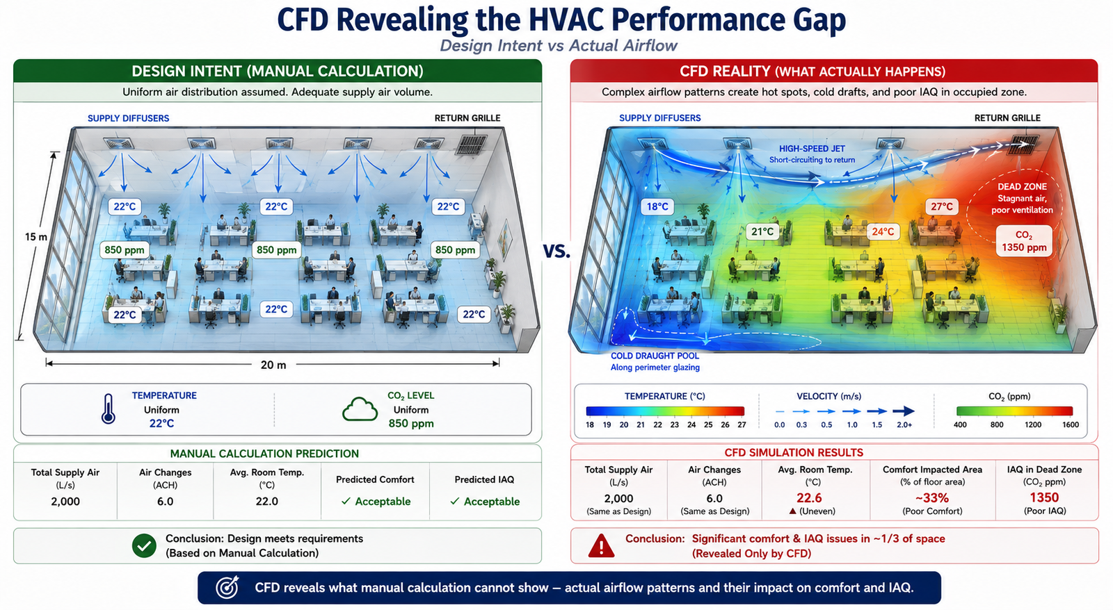
The 15,000 m² office building was designed to meet ASHRAE 55 thermal comfort standards. Mechanical calculations confirmed adequate supply airflow, diffuser throw distances, and a 12 air-change rate in every zone, while BMS commissioning data showed that the fans were delivering the required airflow. Yet six months after occupancy, 34% of occupants rated their thermal comfort as unacceptable. The calculations were correct, but the airflow distribution was not. Two of the eight ceiling diffusers created a Coanda jet that travelled directly toward the return grille, short-circuiting about 12% of the supply air before it reached the occupied zone. A far corner received almost no fresh supply air, resulting in elevated CO₂ levels and uncomfortable conditions.
This illustrates a fundamental HVAC design challenge: correct airflow quantity does not guarantee correct airflow distribution. Manual calculations can determine supply volume, cooling load, and diffuser velocity, but they cannot fully predict how air moves through a complex three-dimensional space. Computational fluid dynamics (CFD) can reveal airflow patterns, temperature distribution, draught risk, short-circuiting, and stagnant zones before commissioning. This article explores the key applications of CFD in HVAC performance, including thermal comfort, duct pressure losses, airflow distribution, cleanrooms, data centres, smoke control, and energy optimization, with practical examples showing how CFD results translate into specific design improvements.
Where CFD Adds Value in HVAC: The Ten Application Areas
CFD is not the right tool for every HVAC engineering task. Sizing a duct run, selecting a chiller, or calculating a heating load are manual calculation tasks where CFD adds no value, the physics is one-dimensional and the established methods are accurate. CFD becomes valuable when the flow is three-dimensional and the interactions between geometry, thermal loads, and airflow patterns determine the outcome. The following table maps the ten HVAC application areas where CFD provides information that manual methods cannot, with the physics, key outputs, design decisions enabled, and fidelity level required.
| HVAC Application | CFD Physics Required | Key Output Metrics | Design Decision Enabled | Fidelity Level |
| Room airflow distribution and comfort | 3D RANS with buoyancy; energy equation for temperature; humidity transport optional | Air temperature at 0.6m, 1.1m, 1.7m above floor; air velocity at occupied zone; draught rate (DR) per ISO 7730 | Diffuser type, location, and throw distance; return grille placement; supply air volume and temperature | Medium, standard RANS k-ω SST; steady-state |
| Duct system pressure drop and flow balancing | 3D RANS in duct network; or 1D network model with CFD-derived loss coefficients | Pressure drop per duct section; flow velocity distribution; balancing damper requirements | Duct sizing, transition geometry, elbow radius, junction design; fan selection and speed | Low to medium, duct segments can be modeled individually; full-network 1D is most efficient |
| Diffuser and grille performance | 3D RANS with fine mesh at diffuser slots; jet throw prediction | Jet throw distance; entrainment ratio; Coanda effect along ceiling; terminal velocity at 0.25 m/s | Diffuser type selection (linear, radial, displacement); supply angle; slot velocity | Medium-High, fine mesh required for slot geometry; validates manufacturer performance curves |
| Chilled beam and radiant cooling | 3D coupled radiation + convection CFD; buoyancy-driven flow | Mean radiant temperature (MRT); operative temperature; natural convection plume from occupants | Chilled beam spacing; supply water temperature; ceiling height requirements | High, radiation model required; occupant thermal plume modelling adds complexity |
| Clean room and ISO class compliance | 3D LES or high-quality RANS; particle transport; filtration efficiency | Air change rate; non-uniformity of velocity; particle concentration; pressure differential to adjacent zones | HEPA/ULPA filter placement; number of air changes per hour; supply/return pattern for ISO 14644 compliance | High, particle tracking and contaminant transport require validated CFD |
| Data centre hot aisle/cold aisle cooling | 3D RANS with server rack power dissipation as volumetric heat source; bypass airflow | Server inlet temperature; rack temperature non-uniformity; bypass ratio (cold air short-circuit); PUE impact | Rack layout; containment design; CRAC unit placement; floor tile perforation pattern | Medium, simplified rack models acceptable; detailed model for hot aisle containment validation |
| Kitchen and laboratory exhaust hood capture | 3D transient or steady RANS; contaminant species transport; thermal buoyancy from cooking source | Capture velocity at hood face; contaminant containment at design flow; spillage under cross-draught | Hood face velocity; exhaust volume flow; makeup air location to avoid cross-draught interference | Medium-High, transient better for intermittent loads; species transport adds cost |
| Hospital operating theatre ventilation | 3D RANS; particle transport; unidirectional flow (UDF) validation | Surgical site air cleanliness; particle counts in critical zone; ISO 14644 zone boundary | UDF canopy dimensions; supply velocity; supply air temperature; recirculation avoidance | High, regulatory compliance requires detailed particle transport validation |
| Natural ventilation / mixed-mode buildings | 3D CFD with wind boundary conditions + buoyancy; external + internal domains coupled | Air change rate; CO2 concentration; thermal comfort metrics (PMV, PPD); wind-driven infiltration | Window opening size and location; stack height; cross-ventilation path; supplementary mechanical system sizing | High, coupled external wind + internal buoyancy requires complex boundary conditions |
| Smoke control and fire safety ventilation | 3D FDS (Fire Dynamics Simulator) or RANS with combustion; species transport; radiation | Smoke layer height; visibility; CO concentration; time to untenable conditions; pressure differential for stairwell pressurisation | Smoke extract fan sizing and location; pressure differential requirements; fire-rated damper locations; egress path validation | High, regulatory requirement for complex buildings; fire codes (NFPA 92, BS EN 12101) specify acceptance criteria |
Thermal Comfort Metrics: What CFD Computes That Calculations Cannot
The thermal comfort metrics defined by ASHRAE 55 and ISO 7730, including PMV, PPD, operative temperature, and draught rate, depend on local conditions at the occupant’s position. These include air temperature, air velocity, turbulence intensity, mean radiant temperature, and relative humidity.
Manual HVAC calculations typically estimate room-average conditions, while CFD can predict the spatial distribution of these parameters throughout the occupied zone. This allows engineers to identify specific areas where thermal comfort criteria are not met, which room-average calculations cannot reveal.
| Comfort Metric | Definition | CFD Output Required | Acceptable Range (ASHRAE 55) | What Poor Performance Looks Like |
| Air temperature at occupied zone | Dry-bulb air temperature at 0.6m (seated) and 1.1m (standing) above finished floor | Temperature scalar field; extract values at specified heights across occupied zone | 20–26°C cooling season; 18–24°C heating season; non-uniformity < 2°C across zone | Stratification > 4°C from ankle to head; cold perimeter pools near glazing; hot spots above equipment |
| Air velocity / draught rate | Mean air velocity at occupied zone; draught rate DR = (34-T_a)(V-0.05)^{0.62}(0.37VT_u+3.14) | Velocity magnitude field; turbulence intensity Tu at occupied zone; extract at grid of points at 0.1m above floor and 1.1m | < 0.15 m/s for sedentary; < 0.25 m/s for light work; DR < 15% per ISO 7730 | High-velocity jets reaching occupied zone from ceiling diffusers; draught from perimeter induction units; floor-level cold air pools |
| Vertical temperature stratification | Temperature difference between ankle level (0.1m) and head level (1.7m) in seated person | Temperature profile from floor to ceiling extracted at multiple room locations | < 3°C ankle-to-head temperature difference per ASHRAE 55 | Displacement ventilation with excessive supply-to-room temperature difference creates > 3°C gradient; hot ceiling / cold floor in cooling mode |
| Mean Radiant Temperature (MRT) | Area-weighted average temperature of all surfaces ‘seen’ by the occupant from their position | Surface temperature field on all enclosure faces; view factor calculation from occupant position | MRT within ±2°C of air temperature preferred; large glazing or exposed hot/cold surfaces can deviate significantly | Winter: cold glazing with U-value > 2.0 W/m²K creates MRT depression; Summer: solar gain through glass creates high MRT even with cool air temperature |
| Predicted Mean Vote (PMV) | ASHRAE/ISO 7730 thermal comfort index from -3 (cold) to +3 (hot); combines air temp, MRT, velocity, humidity, activity, clothing | All above metrics combined in post-processing; requires user metabolic rate and clothing level input | -0.5 to +0.5 for at least 80% of occupants (Category B per ISO 7730) | PMV > +1.0 in summer peak load with undersized cooling; PMV < -1.0 near perimeter in winter heating mode with cold glazing and low-temperature supply air |
| Air change effectiveness (ACE) | Ratio of nominal air change time to actual mean age of air in occupied zone | Mean age of air scalar field computed by solving additional transport equation for air age | > 1.0 for displacement ventilation (plug flow); 0.8–1.0 for mixing ventilation; < 0.5 indicates significant short-circuiting | ACE < 0.5 when supply diffuser is positioned directly above return grille; short-circuit flow bypasses occupied zone entirely |
| CO2 / contaminant concentration | CO2 as proxy for ventilation effectiveness; contaminant dilution from internal sources | Species transport equation for CO2 or contaminant; steady-state concentration field | CO2 < 1000 ppm in occupied zone (ASHRAE 62.1); < 800 ppm for enhanced ventilation | CO2 > 1200 ppm in poorly mixed corner zones not served by supply air; dead zones created by furniture arrangement blocking flow paths |
The Draught Rate Problem: Why High-Throw Diffusers Cause Complaints
Draught, the sensation of unwanted local cooling produced by air movement at velocities above approximately 0.15 m/s at occupant level, is the most frequent comfort complaint in mechanically ventilated offices. The draught rate (DR) formula from ISO 7730 combines air temperature, mean air velocity, and turbulence intensity: DR = (34 – T_a)(V – 0.05)^{0.62}(0.37VT_u + 3.14), where T_a is the air temperature in °C, V is the mean air velocity in m/s, and T_u is the turbulence intensity in percent.
Manual HVAC design uses diffuser throw distance, the distance from the diffuser to the point where jet velocity falls to 0.25 m/s, to determine whether supply air reaches the occupied zone safely. However, this calculation typically assumes an isothermal jet in an open room and may not capture real airflow behavior.
Factors such as the Coanda effect, thermal buoyancy, room geometry, and interaction between multiple diffusers can significantly change the actual airflow path. CFD accounts for these effects and predicts air velocity and turbulence at occupant level, providing the data needed to assess draught risk more accurately.
Mean Radiant Temperature: The Invisible Comfort Driver
Mean radiant temperature (MRT) is the area-weighted average temperature of all surfaces visible from the occupant’s position. It is the dominant thermal comfort parameter in spaces with large areas of cold glass (winter), sunlit surfaces (summer), or radiant heating or cooling systems. Operative temperature, the average of air temperature and MRT, is a better predictor of thermal comfort than air temperature alone, and a space can feel hot even with cool supply air if the MRT from sun-heated surfaces is elevated.
Mean radiant temperature (MRT) depends on both the temperature of surrounding surfaces and their geometric relationship to the occupant. CFD with a radiation model can calculate MRT throughout the room by accounting for surface temperatures and occupant-to-surface view factors.
Manual methods can estimate MRT for simple rooms with uniform surface temperatures, but they become less reliable with complex glazing, shading fins, solar penetration, atria, or radiant panels. For spaces where radiant effects strongly influence comfort, CFD with radiation modeling provides a more detailed way to evaluate thermal comfort.
Duct System CFD: Pressure Drop, Flow Balance, and Loss Coefficients
Duct systems are commonly designed using the equal friction, static regain, or T-method to size duct sections and estimate pressure losses. These methods rely on tabulated fitting loss coefficients from the ASHRAE Handbook, Fundamentals, Chapter 21, covering elbows, tees, wyes, transitions, and grilles.
However, these coefficients are based on controlled test conditions and standard fitting geometries. Real duct systems often differ significantly, with rectangular ducts, high aspect ratios, closely spaced fittings, insufficient upstream development lengths, and modified geometries that may not match the available ASHRAE data. In such cases, the tabulated coefficients may not accurately represent the actual airflow and pressure losses.
CFD fills this gap by computing the actual pressure drop and loss coefficient for the specific fitting geometry in the actual installation condition, including the non-ideal inlet flow profile from the preceding fitting. The table below shows the standard ASHRAE loss coefficients for common duct fittings, the CFD-computed values for the same fittings under typical installation conditions, and the design guidance that CFD reveals.
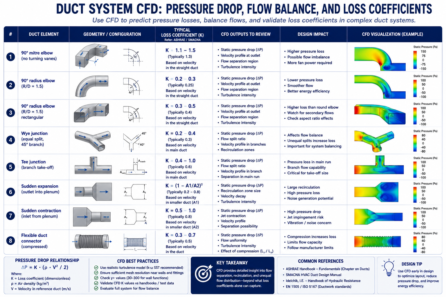
| Duct Element | Loss Coefficient (C or K) | Pressure Drop Formula | CFD vs Standard Value | Design Guidance |
| 90° mitre elbow (no turning vanes) | C = 1.2–1.5 (based on velocity pressure) | ΔP = C × (ρV²/2) | CFD: 1.3–1.5; ASHRAE: 1.2; poor agreement for rectangular ducts | Avoid mitre elbows, use radius elbows (R/D ≥ 1.5) or add turning vanes |
| 90° radius elbow (R/D = 1.5) | C = 0.11–0.15 | ΔP = C × (ρV²/2) | CFD: 0.12–0.14; ASHRAE: 0.11; good agreement at low turbulence intensity | Standard choice for main duct bends; CFD confirms ASHRAE values for round duct |
| 90° radius elbow (R/D = 1.5) rectangular | C = 0.22–0.35 depending on aspect ratio | ΔP = C × (ρV²/2) | CFD reveals 25–40% higher loss than round for same R/D due to secondary flow | Use turning vanes for rectangular elbows with aspect ratio > 2:1 |
| Wye junction (equal split, 45° branch) | C_branch = 0.5–0.8; C_straight = 0.1 | ΔP branch = C × (ρV²/2) of incoming velocity | CFD shows strong sensitivity to branch angle and incoming velocity profile | Ensure uniform velocity approaching junction; reduce branch angle to 30° to lower C_branch |
| Tee junction (branch take-off) | C_branch = 0.9–1.5; C_straight = 0.05–0.2 | Separate C for straight-through and branch | CFD critical here, standard C values assume fully developed upstream flow | Straight duct of ≥ 10 diameters upstream of tee required for ASHRAE C to be valid |
| Sudden expansion (outlet into plenum) | C = 1.0 (full dynamic pressure loss) | ΔP = ρV²/2 (full velocity pressure) | CFD and theory agree well for attached flow; divergence at high expansion ratios | Always add a grille or diffuser cone at duct exit to duct, avoids full dynamic pressure loss |
| Sudden contraction (inlet from plenum) | C = 0.5 (typical); 0.04 for well-rounded inlet | ΔP = C × (ρV²/2) of outlet velocity | CFD shows vena contracta inside duct; rounding inlet reduces C from 0.5 to < 0.1 | Round or bell-mouth duct inlets reduce inlet loss by factor of 5+ vs sharp-edged |
| Flexible duct connector (compressed) | C = 1.5–6.0 depending on compression and bends | ΔP = C × (ρV²/2) | CFD: highly variable; standard values unreliable for compressed flex duct | Keep flex duct fully extended and straight; limit to < 1.8m runs; avoid bends in flex |
Fan Curve Intersection and System Resistance
The fan operating point is determined by where the fan pressure-flow curve intersects the system resistance curve. If the actual system resistance is higher than expected because of underestimated fitting losses or additional bends, the operating point shifts to lower airflow and higher pressure. As a result, the fan may deliver less airflow than the design requires.
CFD can evaluate pressure losses using the as-built duct geometry rather than the original design. For example, replacing a radius elbow with a mitre elbow or placing a branch immediately after a bend can significantly increase system resistance. CFD identifies where the additional pressure drop occurs and helps determine whether balancing dampers or duct modifications are needed to restore the required airflow.
Pressure Balancing in Multi-Branch Systems
In a multi-branch supply duct system, each branch must deliver its design airflow to maintain proper zone performance. Manual balancing dampers are commonly used during commissioning, but they add resistance to the system and can increase the fan’s energy demand. In poorly designed systems, this additional resistance can account for a significant portion of fan power.
CFD optimization can improve flow distribution by adjusting branch sizing, tee angles, and junction geometry so that branches achieve more balanced airflow naturally. By iterating the geometry and pressure losses, engineers can reduce reliance on balancing dampers and avoid unnecessary pressure losses. This approach is particularly useful for complex multi-branch systems where conventional calculations cannot fully capture the detailed pressure distribution at junctions.
Special HVAC Applications: Clean Rooms, Smoke Control, and Data Centres
Clean Room Airflow: ISO 14644 Compliance Through Simulation
Clean room HVAC design must comply with ISO 14644-1, which classifies clean rooms by particle count (ISO Class 1 through 9) and specifies the maximum allowable particle concentration at each class. The air distribution system must deliver clean air to the entire work zone without creating turbulent eddies that could carry particles from less-clean regions into the critical process area. ISO 14644-3 specifically accepts CFD as a method for predicting airflow patterns and validating that the specified air change rate and unidirectionality achieve the required cleanliness class before construction
Cleanroom CFD models typically include the supply HEPA or ULPA filter banks as pressure-drop boundaries, recirculation fan arrays, process equipment as heat sources, operators with metabolic heat output, and low-level return grilles.
The key output is not simply air velocity, but flow unidirectionality, which shows how consistently the supply air moves in the intended direction, typically downward, without excessive lateral mixing. ISO 14644-3 provides criteria for evaluating airflow characteristics. CFD velocity-vector plots across multiple horizontal and vertical planes can reveal whether unidirectional flow is maintained throughout the critical zone or whether recirculation regions could promote particle accumulation.
Smoke Control: CFD for Life Safety Compliance
Smoke control systems in large buildings, atria, underground car parks, shopping centres, airport terminals, must be designed to maintain a clear layer of breathable air below the smoke layer for sufficient time to enable safe evacuation. The performance criteria are defined in fire codes (NFPA 92, BS EN 12101-6, CIBSE Guide E) and typically include: smoke layer height above 2.5 metres from floor level for the first 10 minutes; visibility of at least 10 metres in the clear layer; and CO concentration below 1,500 ppm in the clear layer.
CFD for smoke control uses tools such as Fire Dynamics Simulator (FDS) or general-purpose CFD with combustion and species-transport models. The simulation represents the fire source, its heat-release rate and growth, the rising thermal plume, smoke-layer development, smoke extraction, and make-up airflows.
The main output is the smoke-layer height and clear-layer conditions over time, typically from ignition through the first 20 minutes. This helps engineers determine whether the smoke-control system is adequately sized and where modifications may be needed. Unlike analytical models, which are generally limited to simpler geometries, CFD can evaluate smoke movement in complex building layouts.
Data Centre Hot Aisle/Cold Aisle: CFD as the Primary Design Tool
Data centre thermal management is a critical CFD application because high-density server racks can generate 10–30 kW of heat within a compact footprint. Cold aisle/hot aisle layouts help manage this heat, but real airflow is more complex than the layout suggests. Cold air can bypass unused rack spaces, hot exhaust can recirculate into cold aisles, and airflow from perforated floor tiles can vary because of underfloor pressure differences.
CFD models the data hall, server racks, floor tiles, CRAC units, and underfloor plenum to predict these airflow and temperature patterns. The key metric is the server rack inlet temperature, which must remain within the manufacturer’s specified limit at every rack. CFD also identifies hot spots, cold-air bypass, and hot-air recirculation, helping engineers optimize cooling capacity, improve Power Usage Effectiveness (PUE), and maintain sufficient thermal margin for future capacity increases.
Energy Optimisation: What CFD Enables That Energy Modelling Cannot
Building energy modelling tools such as EnergyPlus, IES-VE, and DesignBuilder simulate building thermal loads and HVAC performance hour by hour throughout the year. They are widely used for energy-code compliance and for predicting annual energy use intensity (EUI).
However, these models typically use simplified, zone-based airflow assumptions and cannot show the detailed airflow distribution within a room. They may therefore be unable to determine whether strategies such as displacement ventilation, natural ventilation, or lower air-change rates can maintain required comfort and indoor air quality. For these decisions, CFD provides the detailed airflow analysis that zone-based energy models cannot.
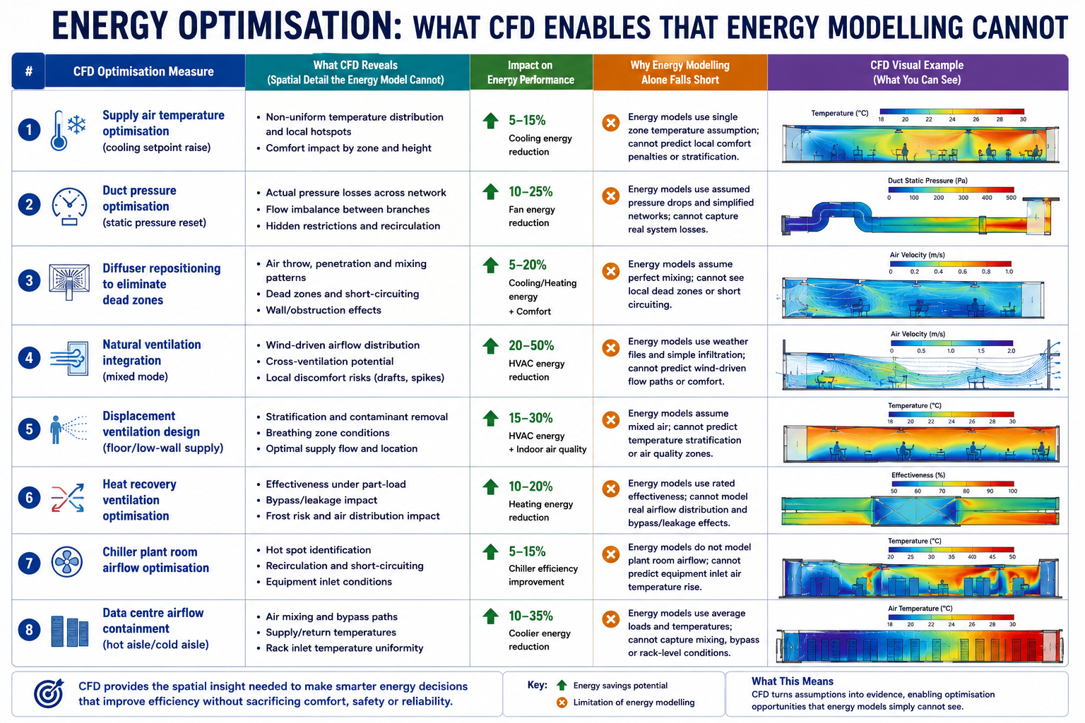
The energy optimisation measures in the table below are enabled by CFD because each one requires confirming that a changed ventilation strategy, lower airflow, higher supply temperature, different distribution, still meets comfort and indoor air quality criteria. Without CFD, the engineer cannot confirm this and must fall back to conservative assumptions that preserve the original over-designed system
| CFD Optimisation Measure | Typical Energy Saving | Mechanism | Payback Period | Best Applicable Building Type |
| Supply air temperature optimisation (cooling setpoint raise) | 5–15% cooling energy | CFD confirms that raising supply air temperature by 1–2°C while repositioning diffusers maintains comfort, reduced chiller lift | Immediate, no capital cost for existing system with variable supply temp | Office, commercial, any VAV system with chiller |
| Duct pressure optimisation (static pressure reset) | 10–25% fan energy | CFD identifies over-pressurised branch circuits; static pressure reset reduces fan speed while maintaining all zones at minimum required pressure | Immediate for VAV systems with BMS; < 6 months for controls upgrade | Any VAV system; largest savings in systems originally set at maximum static pressure |
| Diffuser repositioning to eliminate dead zones | 5–10% ventilation energy | CFD identifies under-served zones requiring extra air volume; repositioning diffusers achieves uniform distribution at lower total airflow | Low capital; repositioning diffusers costs $200–$2,000 per diffuser depending on ceiling access | Open-plan offices; retail; spaces with asymmetric occupancy patterns |
| Natural ventilation integration (mixed mode) | 20–50% cooling energy in mild climates | CFD proves operable window positions and stack effect sizing can meet comfort criteria for 40–60% of operating hours, eliminating mechanical cooling | 3–8 years for window actuator installation; major energy saving for lifetime of building | Office, education, residential in temperate climates; not suitable for humid tropical climates without dehumidification |
| Displacement ventilation design (floor/low-wall supply) | 15–30% ventilation fan energy vs overhead mixing | CFD validates that lower air change rates achieve same air quality due to ACE > 1.0 for displacement vs 0.8 for mixing, less fan power for same IAQ | Premium for displacement diffusers vs ceiling diffusers; ROI 3–7 years in energy costs | High-ceiling spaces: offices, theatres, airports, atriums; not suitable for spaces requiring rapid temperature response |
| Heat recovery ventilation optimisation | 30–50% ventilation heating/cooling energy | CFD models cross-contamination risk in heat exchanger bypass conditions; validates minimum outdoor air rates while maximising heat recovery | Heat recovery units: 3–6 years payback in heating-dominated climates | Any building with high ventilation rates: laboratories, schools, hospitals, commercial kitchens |
| Chiller plant room airflow optimisation | 2–8% chiller energy | CFD of chiller room reveals recirculation of condenser air; repositioning fans or adding baffles reduces condenser entering air temperature by 1–3°C, improving COP | Low capital: baffles $1,000–$10,000; saves 2–5% of chiller energy year-round | Any air-cooled chiller plant; greatest benefit in confined plant rooms with multiple units |
| Data centre airflow containment (hot aisle/cold aisle) | 20–40% cooling energy for data centre | CFD quantifies bypass and recirculation flows; hot aisle containment eliminates mixing; supply air temperature can be raised 5–10°C with same server inlet temperature | 12–24 months typical for hot aisle containment installation in existing data centre | Data centres and server rooms; any high-density electronics cooling application |
Worked Examples: CFD Driving HVAC Design Changes
Example 1: Open-Plan Office, Resolving the Dead Zone
A 400 m² open-plan office floor plate is served by 16 ceiling swirl diffusers at 5m × 5m grid spacing, each supplying 180 L/s at 14°C in cooling mode. The HVAC engineer’s calculation confirmed adequate air change rate (11 ACH) and design throw distance for each diffuser. Post-occupancy surveys showed 28 percent dissatisfaction, concentrated in the two corners farthest from the main supply duct riser.
CFD model: 3D RANS k-ω SST with buoyancy (Boussinesq approximation); 52 million cell mesh resolving diffuser geometry; steady-state; 26 occupants as heat sources at 75W sensible each; 8 workstation computers at 120W each; perimeter glazing as boundary condition at 35°C surface temperature (peak summer).
CFD findings: The two corner zones had air velocities below 0.05 m/s and temperatures of 27.5°C, well above the 24°C design point. Mean age of air in the corners was 42 minutes versus 9 minutes (nominal), indicating that only 21 percent of the design air change rate was being achieved in those zones. The failure mode: the corner diffusers were positioned 2.8m from the perimeter wall, within the Coanda attachment zone. The jets attached to the ceiling and ran parallel to the perimeter wall rather than projecting into the room, then short-circuited to return grilles positioned along the corridor.
CFD-driven design change: Relocate two corner diffusers to 1.2m from the perimeter wall to project jets perpendicular to the glazing, breaking the Coanda attachment and directing air into the unserved zone. Add two additional linear slot diffusers at the perimeter glazing supplying 60 L/s each at 14°C to counteract the solar gain and cold glass convection currents. Reposition one return grille from the corridor side to the interior of the corner zone.
Predicted outcome from CFD: Corner zone temperatures reduced from 27.5°C to 23.8°C. Air velocity in corner zone increased from 0.05 to 0.12 m/s, below draught threshold. PMV in corner zone improved from +1.4 (warm, 34% dissatisfied) to +0.2 (neutral, 6% dissatisfied). Mean age of air reduced from 42 minutes to 11 minutes. Total supply airflow unchanged, comfort achieved by redistribution, not additional air volume.
BEFORE (existing diffuser positions): |
Example 2: Hospital Operating Theatre, Validating Unidirectional Flow
A new 36 m² operating theatre is designed with a 3.4 m × 3.4 m HEPA-filtered unidirectional flow (UDF) canopy supplying 0.36 m/s downward air velocity across the surgical site. The theatre also has peripheral low-velocity induction diffusers around the room perimeter. Building regulations (HTM 03-01 in the UK) require that the critical zone around the operating table maintains ISO Class 5 cleanliness (< 3,520 particles ≥ 0.5μm per cubic metre).
CFD model: 3D RANS; HEPA canopy as uniform velocity inlet; peripheral diffusers as momentum sources; surgical team as heat sources (5 persons at 80W each + 60W metabolic); anaesthetic equipment as obstruction; operating table at body temperature; surgical lights as 400W overhead heat source.
CFD findings: The unidirectional zone was maintained correctly for 80 percent of the canopy area. However, the anaesthetic screen at the head of the table, a vertical partition 1.2m tall running perpendicular to the airflow, created a recirculation zone on the downstream side. The vortex behind the screen carried particles from the periphery of the theatre back into the lower portion of the UDF zone at the incision site. The contamination risk was highest during patient intubation, when the anaesthetic screen was at its maximum height.
Design change: Tilt the UDF canopy 3 degrees toward the head of the table to direct the primary jet slightly away from the anaesthetic screen wake. Add two supplementary slot supply points at the head of the table, supplied from the UDF plenum at 0.15 m/s, to fill the recirculation zone behind the screen with clean air. The supplementary slots are integrated into the anaesthetic equipment mounting rail, no additional ceiling penetrations required.
Outcome: Recirculation zone behind anaesthetic screen eliminated at the incision site level. Particle tracking simulation confirms < 10 particles ≥ 0.5μm per cubic metre at the incision site under worst-case conditions (anaesthetic screen at maximum height, all personnel in position). ISO Class 5 compliance confirmed across the full critical zone. Modification identified before construction, the supplementary slots are built into the equipment rail during factory manufacture at a cost of approximately £800, versus a post-construction modification cost estimated at £15,000 to £25,000 if the problem had been discovered during commissioning testing.
Example 3: Data Centre, Hot Aisle Containment ROI Analysis
A 200-rack data centre hall with 2,000m² floor area is operating at average rack power of 6 kW per rack (1,200 kW total IT load). Current cooling configuration uses 12 CRAC units each rated at 150 kW at 18°C supply. The measured average server inlet temperature is 28°C, within specification but with 15 percent of racks showing inlet temperatures above 30°C at peak load. PUE is 1.72.
CFD findings before containment: Bypass ratio (cold air flowing from cold aisle to hot aisle overhead without passing through racks) was 23 percent of total CRAC supply. Recirculation fraction (hot exhaust air re-entering cold aisle over rack tops) was 18 percent. The combined effect was that 41 percent of cooling capacity was wasted on air that either bypassed the racks or was pre-heated by recirculation before entering the servers.
CFD model of hot aisle containment: Install full height containment doors at the ends of each hot aisle and a solid ceiling above the hot aisle to the raised floor plenum return. All CRAC units relocated to the hot aisle side to take in the warmest air directly. Supply perforated tiles repositioned to ensure uniform cold aisle pressure.
CFD Results After Containment
After hot aisle containment, the bypass ratio decreased from 23% to 3%, while the recirculation fraction dropped from 18% to 2%. Supply air entering the CRAC units increased from an average of 24°C to 34°C, allowing the units to cool directly from the hot aisle rather than a mixed-air environment.
This made it possible to increase the CRAC supply temperature from 18°C to 23°C while maintaining a server inlet temperature of 28°C. The higher supply temperature improved chiller COP by approximately 18%, contributing to a 24% reduction in cooling energy.
For a 1,200 kW IT load operating 8,760 hours per year at $0.12/kWh, the improved PUE from 1.72 to 1.42 results in estimated annual savings of approximately $432,000. With a hot aisle containment installation cost of $180,000, the calculated simple payback is about 5 months.
Building an Accurate HVAC CFD Model: Setup Decisions That Determine Accuracy
HVAC CFD models have specific setup decisions that differ from structural or external aerodynamics CFD. The following covers the most important HVAC-specific decisions that govern result accuracy.
Turbulence Model Selection for HVAC
The RANS k-ω SST model is a common choice for HVAC CFD because it handles wall-bounded flows, supply jets, and room-scale convection at a reasonable computational cost. For typical HVAC temperature differences, the Boussinesq approximation is widely used to model buoyancy. When temperature differences become large or buoyancy dominates, a full variable-density model using the ideal gas law provides greater accuracy.
The k-ε model is also used for HVAC simulations, but it can be less accurate near walls and in regions with strong flow curvature, such as duct bends and diffuser jets. The SST model combines k-ω behavior near walls with k-ε behavior in the free stream, making it suitable for a broad range of HVAC flow conditions.
For natural ventilation and low-velocity spaces, where buoyancy-driven flow and thermal stratification dominate, LES or unsteady RANS may be needed to capture transient flow structures. However, these approaches require significantly more computational resources and are generally reserved for research-grade or compliance-critical analyses.
Diffuser Modelling: The Room Inlet Boundary Condition
Diffusers are the most challenging element of HVAC CFD because their complex internal geometry, slot vanes, swirl blades, perforated faces, cannot be practically meshed in a room-scale simulation without creating a prohibitively large model. Several simplified approaches are used:
- Momentum source method (MSM): The diffuser is replaced by a volumetric momentum source in the cells occupying the diffuser location. The source term injects momentum in the correct direction and magnitude to match the diffuser’s throw and spread. Computationally efficient and accurate for the room-scale flow prediction; less accurate near the diffuser itself.
- Prescribed velocity profile method: A measured or manufacturer-specified velocity profile is applied as an inlet boundary condition at the diffuser face. Requires manufacturer CFD data or physical measurement; more accurate than MSM near the diffuser.
- Simplified box model: A box representing the diffuser envelope is included in the room geometry, with appropriate inlet faces for the supply slots. Requires fine mesh at the diffuser but correctly predicts the near-diffuser flow pattern including Coanda attachment.
For most comfort assessment applications, the momentum source method with manufacturer-specified throw characteristics is adequate and is the standard approach in HVAC-specific CFD software (Flovent, Flomerics, Simscale HVAC). For applications where the near-diffuser flow pattern is critical, theatre ventilation, clean room UDF validation, operating theatre compliance, the simplified box or prescribed profile method is preferred.
Occupant and Equipment Heat Loads
People and equipment are heat sources that drive the thermal plumes and buoyancy currents that govern room airflow in spaces with moderate to low forced convection. The thermal plume from a seated person (sensible heat output approximately 75W) rises at 0.1 to 0.3 m/s and reaches the ceiling in 3 to 5 seconds in a 3m high room, interacting with the ceiling jet from supply diffusers and creating complex mixed convection patterns that no manual method can predict.
In HVAC CFD models, people are typically represented as simplified geometry (a seated or standing cylinder or box) with a specified sensible heat flux on the body surface. The exact shape has less influence on the room-scale flow than the heat flux magnitude and the relative positions of people and supply diffusers. Equipment is represented as block geometries with specified heat dissipation rates. For applications where the precise thermal plume from an individual person or workstation matters (operating theatre, clean room, personal comfort ventilation systems), higher-fidelity occupant models with segmented body heat release are used.
Validating HVAC CFD: When Results Can Be Trusted
HVAC CFD results are more variable in accuracy than external aerodynamics CFD because the buoyancy-driven flows, diffuser jets, and room-scale turbulence are harder to model correctly than attached boundary layers at cruise conditions. The standard validation approach for HVAC CFD is comparison against ASHRAE Standard 129 benchmark cases, a set of generic room configurations with published experimental data for temperature and velocity distributions that CFD codes can be compared against before being applied to real projects.
In addition to benchmark case validation, project-specific validation uses one or more of the following:
- Air temperature measurement: Calibrated temperature sensors at standardised heights (0.1m, 0.6m, 1.1m, 1.7m above floor per ASHRAE 55) at multiple room locations. CFD predictions within ±1.5°C of measured values are considered good agreement for room temperature. Large discrepancies (> 3°C) indicate errors in supply air conditions, thermal load estimates, or diffuser modelling.
- Air velocity measurement: Omnidirectional anemometers at occupied zone locations. Agreement within ±0.05 m/s or 20 percent of measured velocity (whichever is larger) is typical for HVAC CFD. High-velocity regions near diffusers require accurate diffuser modelling for velocity agreement.
- CO2 tracer gas: SF6 or CO2 tracer gas injected at the supply and measured at multiple return and room locations. The tracer gas concentration distribution validates the CFD-computed flow distribution and age-of-air predictions. This is the most sensitive validation for ventilation effectiveness, concentration non-uniformities that temperature measurements miss are revealed by tracer gas.
- Smoke visualisation: Theatrical smoke or titanium tetrachloride smoke bombs reveal the actual flow pattern in a room, showing jet directions, recirculation zones, and dead zones. Not quantitative but provides immediate qualitative confirmation of the CFD-predicted flow pattern, or reveals patterns that the CFD model did not predict, indicating modelling errors to correct.
Frequently Asked Questions
Q: Can CFD replace manual HVAC design calculations?
No. CFD complements manual HVAC calculations rather than replacing them. Manual methods determine loads, airflow, duct sizing, pressure drops, and equipment selection, while CFD evaluates how air actually moves through the space, including temperature distribution, occupant comfort, and draught risk. The best approach is to use manual calculations for system sizing and CFD for airflow distribution validation and optimization.
Q: What is the Coanda effect and why does it matter for HVAC diffuser design?
The Coanda effect causes a fluid jet to remain attached to a nearby surface. In HVAC, ceiling-mounted supply jets can attach to the ceiling and travel farther across the room before dropping into the occupied zone, helping reduce draughts. However, excessive attachment can carry the jet past its intended path and cause short-circuiting or dead zones near return grilles and perimeter walls. CFD can predict how jet momentum, supply temperature, and ceiling geometry affect Coanda attachment and detachment, which simplified throw-distance calculations cannot fully capture.
Q: How does CFD help with HVAC energy optimisation?
CFD enables HVAC energy optimization by confirming that lower-energy operating strategies still meet thermal comfort and indoor air quality requirements. For example, raising supply air temperature from 13°C to 16°C can improve chiller efficiency, but it also changes jet buoyancy, Coanda attachment, and occupied-zone temperature distribution. CFD can verify whether comfort is maintained before the change is implemented. If the criteria are met, the higher setpoint can reduce cooling energy without major capital changes.
Q: What is air change effectiveness and how does CFD compute it?
Air change effectiveness (ACE) measures how effectively fresh supply air reaches the occupied zone. An ACE of 1.0 represents ideal mixing, while values above 1.0 indicate more effective air delivery, such as displacement ventilation. Values below 1.0 indicate poor distribution or short-circuiting between supply and return air.
CFD calculates ACE by tracking the age of air throughout the room using an additional transport equation. This provides the local and zone-average air age and shows where fresh air reaches occupants efficiently or where it is bypassing the occupied zone. Because ACE depends on the full three-dimensional airflow field, it cannot be accurately determined from conventional manual HVAC calculations alone.
Q: How accurate is HVAC CFD compared to physical measurement?
HVAC CFD accuracy depends on the application and model quality. For forced-convection rooms, temperature predictions are typically within ±1.5–3°C and occupied-zone velocity within ±0.03–0.08 m/s of measurements. Naturally ventilated spaces can have larger temperature errors of ±3–5°C, while CO₂ predictions are typically within 10–20% when airflow distribution is accurately captured. For code compliance, CFD should be validated against benchmark data or physical measurements.
Q: When is HVAC CFD required rather than just beneficial?
HVAC CFD becomes essential in four situations: regulatory compliance for applications such as operating theatres, smoke control, and cleanrooms; complex or non-standard geometries such as atria and large open halls; mixed-mode or natural ventilation, where wind and buoyancy-driven flows interact; and post-occupancy problems, where CFD can identify airflow deficiencies in an as-built system and guide targeted corrective measures instead of trial-and-error adjustments.
Conclusion: CFD as the Design Verification Tool for HVAC Performance
HVAC systems can be correctly sized using established manual calculation methods, yet still fail to perform as expected when supply air does not reach occupants at the right quantity, temperature, and velocity. The actual distribution of airflow and temperature depends on three-dimensional effects such as Coanda attachment, buoyancy plumes, furniture and partitions, and supply-to-return short-circuiting. CFD captures these effects and can identify comfort problems, CO₂ accumulation, inadequate diffuser throw, and airflow deficiencies before commissioning. This makes CFD particularly valuable when air distribution directly affects building performance and occupant comfort.
The strongest approach is to use manual calculations for HVAC system sizing and CFD for airflow distribution validation and optimization. CFD can also support energy-saving strategies such as higher supply temperatures, lower air-change rates, displacement ventilation, and hot aisle containment. By identifying problems and testing design changes before construction or commissioning, CFD can reduce costly remediation, improve occupant comfort, and help HVAC systems perform as designed from day one.
Explore related simulation topics: thermal simulation in electronics, CFD vs wind tunnel testing, static vs dynamic analysis, why simulation fails, and how leading industries deploy simulation to improve performance and reduce cost.