The geometry was perfect. It had been built by an experienced CAD designer who understood the manufacturing process, modeled every fillet to the correct radius, and exported a clean, watertight solid body that meshed without errors. The mesh quality metrics were excellent, Jacobian above 0.85, aspect ratio below 4:1 throughout, convergence confirmed with three mesh refinements. The boundary conditions matched the physical test setup. The material properties were from the certified material datasheet. Every box on the preprocessing checklist was checked.
The simulation predicted a maximum stress of 187 MPa at the shaft shoulder. The shaft yielded at 220 MPa. The safety factor appeared to be 1.18, adequate for a non-critical application. The shaft failed in fatigue after 80,000 cycles. The laboratory fatigue test, run afterward to investigate the failure, showed a fatigue life of 85,000 cycles, consistent with the physical failure. The simulation had predicted 187 MPa of peak von Mises stress.
The fatigue analysis used that number. What neither the simulation setup nor the fatigue analysis had accounted for was that the correct fatigue-driving stress was the signed maximum principal stress amplitude, and under the combined bending and torsion loading, the maximum principal stress amplitude was 312 MPa, not 187 MPa. The safety factor was not 1.18. It was 0.71.
The failure was not caused by bad CAD. It was not caused by a mesh problem. It was not caused by wrong boundary conditions or incorrect material properties. It was caused by misidentifying which stress quantity drives fatigue failure, a postprocessing interpretation error that is entirely independent of the quality of the CAD model, the mesh, or any other preprocessing decision. This is the central reality of simulation accuracy: the overwhelming majority of simulation failures occur in the decisions the analyst makes about physics, modeling approach, and results interpretation, not in the geometric representation of the part.
This article catalogs the twelve categories of simulation failure beyond geometry quality, provides the complete physics assumption error table for structural FEA, the eight most common postprocessing interpretation mistakes and how to avoid them, and the validation methods that catch errors before they propagate to wrong design decisions. The goal is a framework for understanding why simulation fails when the CAD model is not the problem, which is most of the time.
The Complete Taxonomy of Simulation Failure
Simulation failure, producing a result that does not represent the physical behavior of the structure, occurs at four distinct layers: physics and modelling decisions, preprocessing decisions, solver numerics, and postprocessing and interpretation. CAD geometry quality is a subset of preprocessing decisions and, when it is the problem, it typically manifests as mesh generation failure (which is obvious) or poor mesh quality (which is caught by quality metrics). The subtle failures, the ones that produce plausible-looking wrong results, occur almost entirely in physics assumptions and postprocessing interpretation, two layers that are completely independent of CAD quality.
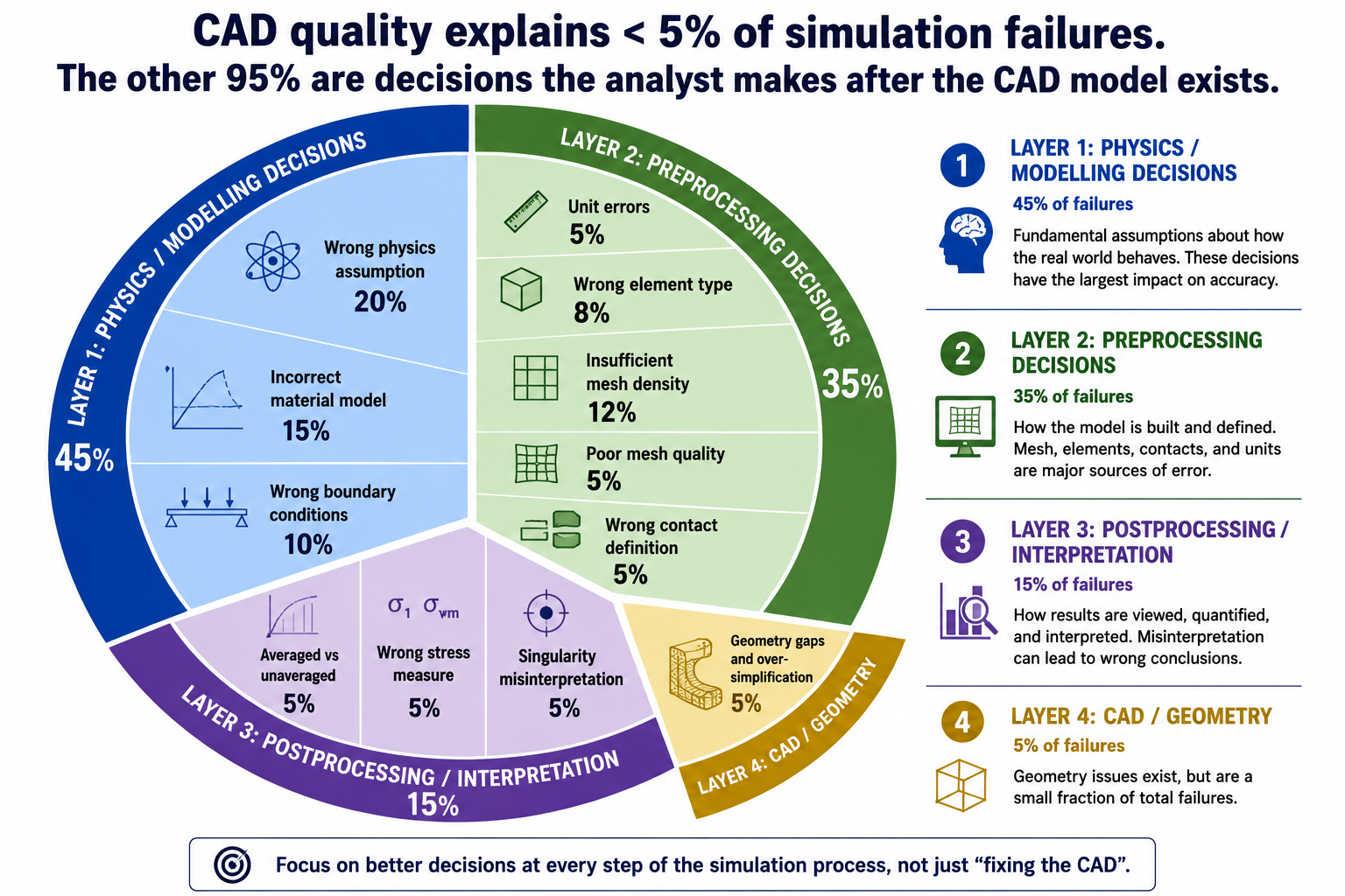
| Failure Category | Root Cause Layer | CAD Quality Relevant? | Typical Error Magnitude | Detection Method |
| Wrong physics assumption | Modelling, analyst decision | No | 50% to orders of magnitude, depends on how wrong the physics model is | Comparison with analytical solution or independent simulation using different physics |
| Incorrect material model | Modelling, data input | No | 5% to 10x, linear vs nonlinear material can differ by factor of 3-10 at high loads | Material model sensitivity study; comparison with coupon test data |
| Wrong boundary conditions | Modelling, analyst decision | No | 20% to 10x, fixed vs pinned changes bending moment distribution completely | BC sensitivity study; reaction force equilibrium check; deformation shape inspection |
| Incorrect load definition | Modelling, analyst decision | No | Up to 100%, wrong direction inverts sign of all results; wrong area changes magnitude proportionally | Load verification against specification; reaction sum check |
| Unit system inconsistency | Preprocessing, data entry | No | Factor of 10^3 to 10^9, material property in wrong units | Unit verification test (cube under unit load); modal frequency check |
| Wrong element type | Preprocessing, analyst decision | No | 10% to 50%, TET4 vs TET10 at stress concentrations; shell vs solid for thick sections | Element sensitivity study; compare with known analytical solution |
| Insufficient mesh density | Preprocessing, analyst decision | No | 5% to 40% at stress concentrations without convergence study | Mesh convergence study; compare peak stress across three mesh refinements |
| Poor mesh quality | Preprocessing, mesh generation | Partially, bad CAD produces bad meshes | 5% to 30% from Jacobian and aspect ratio degradation | Mesh quality metrics check (Jacobian, aspect ratio, warpage) before solve |
| Missing geometry features (over-simplification) | Preprocessing, geometry | Partially, depends on what was removed | 10% to 5x, removing a load-path fillet removes the stress concentration entirely | Compare simplified model stress with full-geometry model at critical features |
| Incorrect contact definition | Preprocessing, analyst decision | No | 10% to complete loss of load transfer, gap in contact allows interpenetration | Contact force output; check interface stress continuity; gap inspection |
| Numerical solver error (ill-conditioning) | Solver, numerical | No | Small to large, depends on conditioning number of stiffness matrix | Condition number check; residual force check; solver diagnostic output |
| Misinterpretation of results | Postprocessing, analyst decision | No | Up to 100%, von Mises used when principal stress is needed; averaged vs unaveraged stress | Results interpretation protocol; independent reviewer; hand calc comparison |
The most important column in this table is the third: ‘CAD Quality Relevant?’, which is ‘No’ for ten of twelve failure categories. Nine of the twelve failure categories are entirely independent of the CAD model quality. The two categories where CAD quality is partially relevant (poor mesh quality and missing geometry features from over-simplification) can also arise from analyst decisions independent of the original CAD. The implication is direct: improving CAD quality addresses at most 5 to 10 percent of the sources of simulation failure. The other 90 to 95 percent require better physics judgment, more rigorous preprocessing practice, and more systematic results validation.
Category 1: Physics Assumption Errors, The Most Consequential Failures
Physics assumption errors are the simulation failures that produce the largest discrepancies between predicted and actual behavior. They occur when the analyst selects an analysis type, material model, or physical representation that is fundamentally inappropriate for the actual physics of the problem. Unlike mesh density errors, which typically produce 5 to 40 percent discrepancies that systematic mesh refinement will reveal, physics assumption errors can produce results that are wrong by factors of 2 to 50 or more, with no indication from the solver that anything is amiss
The solver cannot detect a physics assumption error. If the analyst sets up a linear elastic static analysis for a structure that actually yields, creeps, and collapses dynamically, the solver applies linear elastic statics faithfully and returns a result that is internally consistent with those assumptions. The result looks exactly like a valid FEA output. The error is in the question that was asked, not in the computation of the answer
| Wrong Assumption | What It Misses | Correct Approach | How to Detect |
| Linear elastic material when plastic deformation occurs | Stress redistribution after yielding; residual stresses; collapse load prediction | Nonlinear material model with isotropic or kinematic hardening | Check if any element von Mises stress exceeds yield, if so, linear analysis is invalid at those locations |
| Static analysis when load is dynamic | Inertia amplification (DAF up to 50x at resonance); resonance; transient effects | Modal analysis to find natural frequencies; harmonic or transient analysis | Calculate frequency ratio f_load/f_nat, if > 0.3, dynamic analysis required |
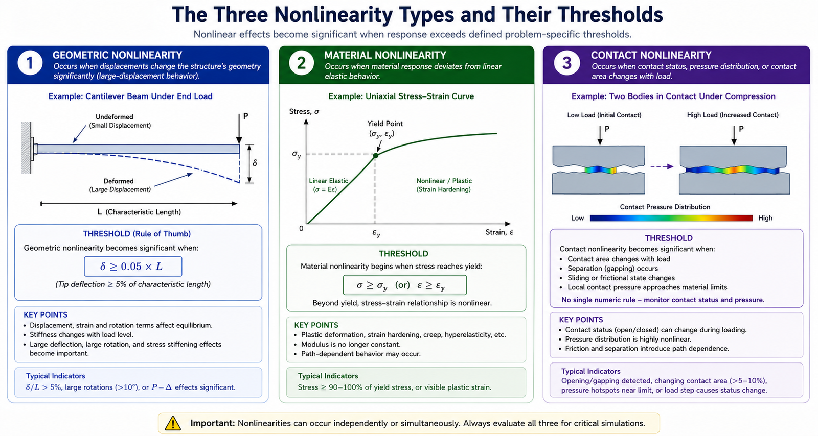
| Small displacement (linear geometry) when deformation is large | Geometric stiffening (cables, membranes); change in load direction with deformation; snap-through instability | Nonlinear geometry (large displacement) analysis | Check if peak displacement exceeds ~5% of characteristic structure dimension |
| Isotropic material for composite or anisotropic structure | Direction-dependent stiffness and strength; interlaminar shear; ply-by-ply stress | Orthotropic or anisotropic material model with correct fiber orientations | Check material data, if E varies by direction, isotropic is wrong |
| Frictionless contact when friction governs load transfer | Friction force component; load distribution change with friction; stick-slip behavior | Frictional contact with measured or estimated friction coefficient | Check if tangential force at interface is significant relative to normal force |
| Room temperature material properties for elevated temperature service | Stiffness reduction (steel: -30% at 400°C); yield stress reduction; creep at sustained high temperature | Temperature-dependent material properties; separate thermal analysis to determine temperature field | Check operating temperature, if > 200°C for steel or > 100°C for aluminum, temperature effects are significant |
| Perfect bond at all interfaces (all tied contact) | Partial separation; interface slip; peel stress at bond terminations; delamination in composites | Contact with separation allowed; cohesive zone model for bond/adhesive | Check if interface peel or shear stress exceeds adhesive or bond strength |
| Single load path (ignoring redundancy or alternative paths) | Load redistribution after local yielding; progressive failure sequence; fail-safe load paths | Nonlinear analysis capturing load redistribution; or explicit multi-path structural model | Check if structure has any redundancy, if hyperstatic, linear analysis misses redistribution |
The Linear Elastic Trap: When Yielding Changes Everything
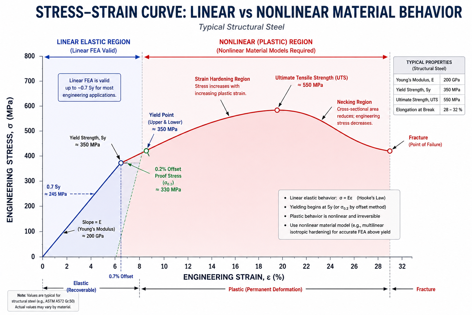
The most common physics assumption error in industrial FEA is the application of linear elastic analysis to structures that yield locally under the applied loads. In linear elastic analysis, stress is proportional to strain everywhere, there is no yielding, no stress redistribution after yielding, and no limit on how high the stress can go. When an element in the model reaches the yield stress, the linear analysis simply continues computing higher stresses as if the material were still elastic.
In ductile materials, local yielding at a stress concentration does not usually cause immediate failure. Instead, the yielded region redistributes load to the surrounding elastic material, limiting the peak stress to approximately the yield strength (plus any strain hardening) and allowing the structure to carry additional load. As a result, linear elastic FEA is conservative for local stress prediction because it can predict stresses above the material’s yield strength, but non-conservative for overall structural behavior because it ignores the beneficial load redistribution that occurs after yielding. Using linear elastic stress results for fatigue analysis in components that experience local yielding can therefore produce misleading results by overestimating local stresses while failing to capture the actual stress distribution.
Large Displacement Effects: When Geometry Changes Under Load
Linear FEA assumes that displacements are small relative to the structure’s dimensions, specifically, that the displaced configuration is so close to the undeformed configuration that the stiffness matrix computed for the original geometry remains valid throughout the loading. This assumption breaks down when displacements exceed approximately 5 percent of the characteristic structural dimension.
Ignoring large displacement effects can produce fundamentally incorrect results. In cables and membranes, geometric stiffening from tension creates the structure’s load-carrying stiffness, which linear analysis cannot capture. In slender columns, geometric softening leads to buckling, while in shallow arches and buckled plates, it governs snap-through instability. These critical behaviors are only predicted with geometric nonlinear analysis.
Temperature Effects: The Invisible Load
Thermal stress is one of the most systematically ignored physics effects in structural FEA. When a structure operates at elevated temperature, or when temperature varies across the structure (as in a heat exchanger, an engine component, or a solar panel), the differential thermal expansion between constrained regions produces stress that can be comparable to or larger than the mechanical stress from applied loads. A steel component that is mechanically unstressed but subjected to a temperature difference of 100°C across a constrained length generates thermal stress of approximately E x alpha x delta_T = 210,000 x 12e-6 x 100 = 252 MPa, close to the yield stress of mild steel, from thermal load alone.
The error of ignoring thermal stress is particularly dangerous in systems that operate under combined mechanical and thermal loading. A pressure vessel at room temperature may have a mechanical stress of 150 MPa against a yield stress of 350 MPa, a safety factor of 2.3. The same vessel at 350°C may have a yield stress of 250 MPa (elevated temperature reduction) plus a thermal stress from the temperature gradient of 100 MPa, reducing the margin to: 350 – 150 – 100 = 100 MPa remaining against 250 MPa yield, an effective safety factor of 1.67 rather than 2.3, and a reduction the mechanical-only analysis would never reveal.
Category 2: Material Model Errors, When the Wrong Data Drives the Analysis
Material model errors span two distinct failure modes: using the wrong material model type (linear elastic when the material is nonlinear, isotropic when it is anisotropic) and using wrong material data values within the correct model type. Both produce results that are wrong but internally consistent, the solver is computing correctly, but it is computing the response of a different material than the one in the actual structure.
The Datasheet vs Design Allowable Distinction
Material datasheets report properties measured on laboratory specimens under idealized conditions: polished surface finish, controlled grain direction, room temperature, no stress concentrations. These are not the design allowable values for structural components. The design allowable, the property value that should be used in a structural analysis to achieve a specified probability of failure, is lower than the datasheet nominal value by factors that account for material variability, environmental effects, product form differences (plate vs forging vs casting), and surface finish.
In aerospace, material allowables are defined by the MMPDS as A-basis (99% population with 95% confidence) and B-basis (90% population). These values are often 10–40% lower than nominal datasheet properties to account for material variability. Using nominal values instead of certified allowables in safety-critical FEA can produce non-conservative results and compromise structural integrity.
Weld and Heat-Affected Zone Properties
Welded structures present a material modeling challenge that is systematically underestimated: the weld metal and the heat-affected zone (HAZ) adjacent to the weld have different mechanical properties from the parent material. For structural steels, the HAZ may have lower toughness than the parent plate (due to heat-induced grain coarsening) while having similar or slightly higher yield stress. For aluminum alloys, the HAZ is typically significantly weaker than the parent material, the peak hardness in the HAZ of a 6061-T6 weld can be 50 percent of the parent material value, equivalent to the O (annealed) temper.
FEA models of welded structures that assign parent material properties to the entire geometry, including the weld zone and HAZ, overestimate the strength at the weld and underestimate the failure risk at the heat-affected zone. For aluminum welded structures in particular, the correct approach is to model the HAZ as a separate material zone with reduced properties, sized according to the heat input and the material’s heat treatment response. The width of the softened HAZ in 6061-T6 aluminum is typically 15 to 25mm on each side of the weld centerline.
Category 3: Boundary Condition and Load Errors, Same Model, Different Answer
Boundary condition and load errors are addressed in the dedicated boundary conditions article, but their contribution to simulation failure deserves emphasis in the context of CAD-independent failures. A model with perfect CAD geometry, excellent mesh quality, and correct material properties can produce results that are wrong by a factor of 2 to 10 if the boundary conditions do not represent the physical support behavior
The most instructive example is the simply supported vs fixed-end beam. Both models have identical CAD geometry and material. The simply supported model (pin at one end, roller at the other) has a maximum bending moment at midspan of wL²/8 and zero moment at the supports. The fixed-fixed model has a maximum moment at the supports of wL²/12 and a midspan moment of wL²/24. For the same distributed load w and span L, the peak moment, and therefore the peak stress, differs by a factor of 3 between the two cases. Which result is correct depends entirely on how the physical supports behave, not on the CAD geometry of the beam.
The Over-Constraint Failure Mode
Over-constraint, applying more constraint than the physical support provides, is the boundary condition error that produces results that appear reasonable but are systematically wrong in a non-conservative direction. A fixed support at a bolted joint adds artificial bending resistance that the bolts do not provide. A fully tied contact at an interface that is actually bonded only in compression prevents the interface separation that would occur in the physical structure under peel loading.
The insidious feature of over-constraint errors is that the model produces lower stresses than the correctly constrained model, it appears to show a healthier safety factor. The fixed end of the over-constrained beam carries a bending moment that does not exist in the physical simply-supported beam, and this phantom moment reduces the midspan stress below the physically correct value. The analyst sees a ‘safe’ result and approves the design, while the physical structure, which does not have the phantom fixed-end moment, carries the full midspan moment that the over-constrained model suppressed.
Distributed vs Point Load Errors
The distribution of applied loads across a surface governs the local stress field near the load introduction zone. A point force applied to a single node produces a mathematically infinite stress at that node, a singularity with exactly the same character as the re-entrant corner singularity. The stress at the loaded node grows without bound as the mesh is refined, never converging to a physical value. This is not a mesh problem, it is a load modeling problem. The physical load is always distributed over a finite contact area, never concentrated at a mathematical point.
The fix is to apply the load over its actual physical contact area: a distributed pressure or traction over the bearing face, rather than a concentrated force at a node. For loads introduced through small contact areas (bolt heads, pin bearings, rivet heads), the contact area must be represented geometrically and the load distributed over that area. If the contact area geometry is too small to mesh explicitly, a remote force with an appropriate coupling constraint distributes the load over a representative surface while maintaining the correct resultant force and moment.
Category 4: Contact Modeling, The Nonlinear Physics That Linear Models Miss
Contact between surfaces is inherently nonlinear: surfaces either touch and transmit force, or they separate and transmit nothing. This binary on-off behavior cannot be represented by a linear model, and yet many structural FEA setups in industrial practice handle multi-component assemblies with either bonded contact (all surfaces permanently touching) or no contact at all (surfaces free to interpenetrate), both of which misrepresent the actual physics for any interface that may partially separate or slide under load.
Bonded Contact: When It’s Right and When It’s Dangerously Wrong
Bonded contact should only be used when surfaces are permanently joined (such as welded or adhesively bonded) and cannot separate or slide under load. If separation or sliding is possible, a contact model should be used instead. Modeling these interfaces as bonded can hide stress concentrations and produce inaccurate load paths, leading to non-conservative FEA results.
The consequence of using bonded contact at an interface that physically separates is that the model misses the peel stress concentration at the separation front, the stress intensity that drives delamination in composites, adhesive bond failure, and fatigue cracking at interference-fit edges. These are real failure modes in physical structures that the bonded contact model cannot predict regardless of how accurately the CAD geometry represents the interface.
Contact Pressure Distribution: Why Linear Models Get Hertzian Contact Wrong
When two curved surfaces contact under load (a ball bearing race, a cam follower, a gear tooth), the contact pressure distribution follows the Hertzian contact theory, a non-uniform pressure distribution across the contact ellipse that is highly concentrated at the center and drops to zero at the contact edge. This distribution can only be correctly predicted by a nonlinear contact model that allows the contact zone to grow as load increases and computes the pressure distribution from the actual surface deformation.
A linear elastic model with bonded contact over an assumed contact area produces a uniform pressure distribution that misrepresents the actual Hertzian distribution by a factor of up to 1.5 at the contact center and is wrong in both sign and magnitude at the contact edge. For applications where contact pressure drives fatigue (rolling contact fatigue in bearings, gear tooth fatigue, cam follower wear), a nonlinear contact analysis with realistic surface geometry and contact formulation is mandatory, the linear bonded contact result is not just inaccurate, it is qualitatively wrong in its prediction of the fatigue-critical stress distribution.
Category 5: Postprocessing Errors, Getting Wrong Answers from Correct Simulations
Postprocessing errors are the failure mode that the FEA preprocessing checklist and the physics assumption review cannot prevent, because they occur after the solver has produced correct results. The solver computes the correct stress tensor at every integration point for the given model setup. The error occurs when the analyst extracts, displays, or interprets those correct results in a way that misrepresents the physical stress state. A simulation that is set up correctly and solved correctly can still fail, by reporting the wrong number for the right location, or the right number for the wrong location, or a result that is correct for one physical interpretation but applied to a different one.
| Error Type | What the Analyst Does | Why It’s Wrong | Correct Approach |
| Using averaged nodal stress instead of unaveraged at stress concentrations | Reports the smoothed, averaged stress contour value at the peak stress node | Averaging blends the peak node value with lower-stressed adjacent nodes, reducing the apparent peak by 10-40%, the true peak is in the unaveraged result | Always extract stress at stress concentration locations from unaveraged (element) results; use averaged results only for smooth stress regions |
| Using von Mises stress for fatigue analysis | Reports peak von Mises as the fatigue-driving stress | Von Mises is a scalar equivalent stress for yield prediction, it has no sign and cannot represent the tension-compression cycle that drives fatigue. Fatigue is driven by the maximum principal stress amplitude | Use signed maximum principal stress or critical plane methods for fatigue; von Mises for yield check only |
| Reporting stress at support nodes as peak stress | Identifies a high stress spike at a constrained node as the design-critical location | Point constraints create mathematical stress singularities that grow without bound as the mesh is refined, they do not converge to a physical value and are not representative of real stress | Exclude support nodes from peak stress evaluation; extract results at least one element size away from point constraints; distribute constraints over a surface |
| Ignoring stress singularities at re-entrant corners | Reports a very high stress at a sharp 90-degree internal corner as the critical stress | Stress at a perfectly sharp re-entrant corner is theoretically infinite in linear elastic FEA, it is a mathematical singularity caused by the corner geometry, not a physical failure prediction | Add a realistic fillet radius at the corner; if the corner must be sharp in the design, use a conservative Kt factor from Peterson’s rather than the singularity value |
| Confusing local and global coordinate stress components | Reports sigma_x from global coordinate system at an inclined surface and compares to material strength in the thickness direction | Stress components are coordinate-system dependent, sigma_x in global coordinates is not the same as the normal stress perpendicular to an inclined surface | Transform stress to the local material coordinate system at the critical surface; use principal stresses for coordinate-independent comparison to material limits |
| Selecting the wrong stress measure for the material failure criterion | Uses von Mises stress to check a brittle ceramic or cast iron component | Von Mises (distortion energy) criterion is appropriate for ductile metals. Brittle materials fail in tension, the maximum principal stress (Rankine) criterion is correct | Match the failure criterion to the material: von Mises for ductile metals; maximum principal stress for ceramics, glass, and gray cast iron; Tsai-Wu or Hashin for composites |
| Reporting maximum stress across entire model without checking location | States ‘maximum stress is 450 MPa’ without reporting where it occurs | The maximum stress location determines whether it represents a real failure risk or a modeling artifact (singularity at a constraint, mesh-dependent peak at a sharp corner) | Always report stress with location: ‘Maximum stress is 450 MPa at the shoulder fillet, r=2mm, confirmed converged with mesh study’ |
| Missing fatigue mean stress correction | Applies Basquin S-N curve directly to stress amplitude without considering mean stress | S-N curves are typically generated at zero mean stress (fully reversed, R=-1). Non-zero mean stress reduces fatigue life, the Goodman or Morrow correction must be applied when mean stress is non-zero | Apply Goodman or Morrow mean stress correction: (sigma_a/Se) + (sigma_m/Su) = 1/SF for Goodman |
The Averaged vs Unaveraged Stress Decision
Every FEA postprocessor offers the choice of displaying stress as averaged nodal stress or unaveraged (element) stress. The difference is significant at stress concentration locations and is the source of one of the most systematic result under-predictions in structural FEA practice.
Averaged nodal stress is computed by averaging the stress values from all elements sharing each node. This averaging smooths the stress field and produces visually cleaner contour plots. At stress concentration locations, where the stress gradient is steep, the peak element has a higher stress than the surrounding elements. The averaging operation blends the peak element’s stress with its lower-stressed neighbors, reducing the displayed peak stress by 10 to 40 percent compared to the true unaveraged value
Unaveraged stress displays the stress for each element from its own integration point extrapolation, without blending with adjacent elements. At a well-meshed stress concentration with sufficient element density, the maximum unaveraged stress converges to the true stress concentration value as the mesh is refined. For all stress extraction at stress concentrations and failure-critical locations, unaveraged element stress is the correct quantity to report. Averaged stress is appropriate for smooth stress field regions where the gradient is small, and for comparing results across a large model at a global level, never for peak stress quantification at a notch, fillet, or hole.
The Stress Singularity Identification Protocol
A stress singularity in FEA is a location where the computed stress grows without bound as the mesh is refined, a sign that the mathematical model has a point of theoretically infinite stress that has no physical counterpart. Not every high-stress node in an FEA model represents a real structural risk, many are singularities caused by modeling choices that must be identified and excluded from design evaluation.
The three most common sources of stress singularities are:
- Sharp re-entrant corners: A 90-degree internal corner in a solid model has theoretically infinite stress in linear elastic FEA. The singularity arises from the corner geometry, not from a physical stress concentration in the real part (which always has a finite radius). Resolution: add the actual corner radius to the model. If the physical corner is truly sharp (ground to a sharp edge), use a stress concentration factor from Peterson’s rather than the FEA singularity value.
- Point constraints: A fixed BC applied to a single node concentrates the reaction force at a mathematical point, producing a stress singularity with exactly the same character as the corner singularity. Resolution: apply BCs over a surface, not a single node; or extract stress results at a distance of at least one element size from the constrained node, where Saint-Venant’s principle ensures the singularity has decayed.
- Point loads: A concentrated force at a single node produces a stress singularity at that node. Resolution: distribute the load over the actual contact surface, or use a remote force with a coupling constraint to a representative load introduction area.
The diagnostic test for a stress singularity: refine the mesh at the suspect location and observe whether the peak stress increases. If the peak stress increases with mesh refinement and shows no sign of converging, it is a singularity. A genuine physical stress concentration converges, the peak stress approaches a finite value as the mesh density increases. A singularity diverges. This distinction is fundamental to correct results interpretation and must be made before reporting any very high stress value from an FEA model.
The Validation Framework: Catching Failures Before They Reach Design Decisions
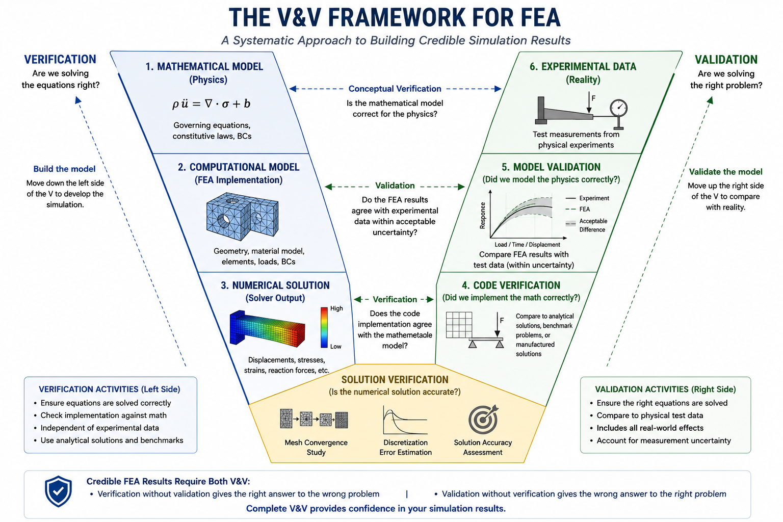
FEA validation is the systematic process of confirming that a simulation result correctly represents the physical behavior of the structure. Validation is not a single check, it is a layered framework of independent verification methods, each of which catches a different class of failure. No single validation method catches all failure modes. A reaction force check does not catch a material model error. A mesh convergence study does not catch a physics assumption error. A hand calculation comparison does not catch a postprocessing interpretation error. All must be applied.
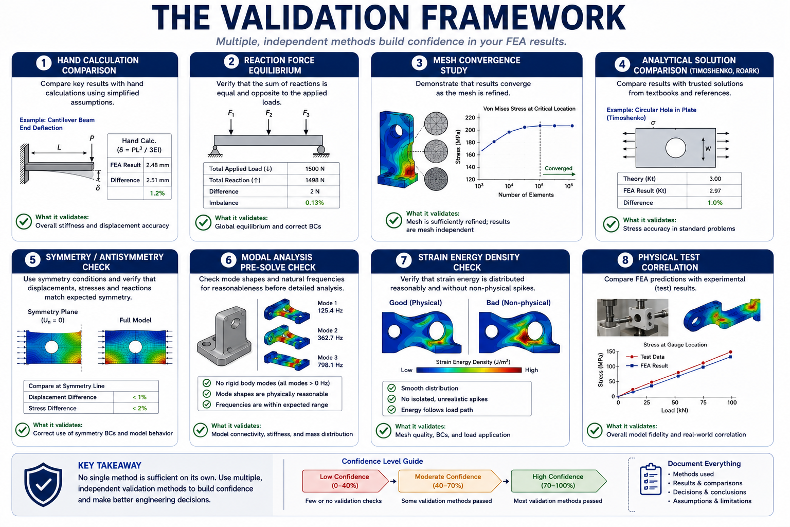
| Validation Method | What It Checks | When to Use | Pass Criterion |
| Hand calculation comparison | Order-of-magnitude correctness of displacement and stress; basic load path logic | Always, every analysis, every load case | FEA result within 20-30% of simplified hand calc; differences explained by geometry complexity, not errors |
| Reaction force equilibrium | Applied loads are correctly transmitted through the model; no load is lost or multiplied at interfaces | Every static analysis as a mandatory post-solve check | Sum of all reaction forces equals sum of all applied forces in each global direction, within 0.1% tolerance |
| Mesh convergence study | Peak stress at critical locations is mesh-independent (converged) | Every analysis where peak stress at a stress concentration governs the design | Peak stress changes < 2% between medium and fine mesh refinements |
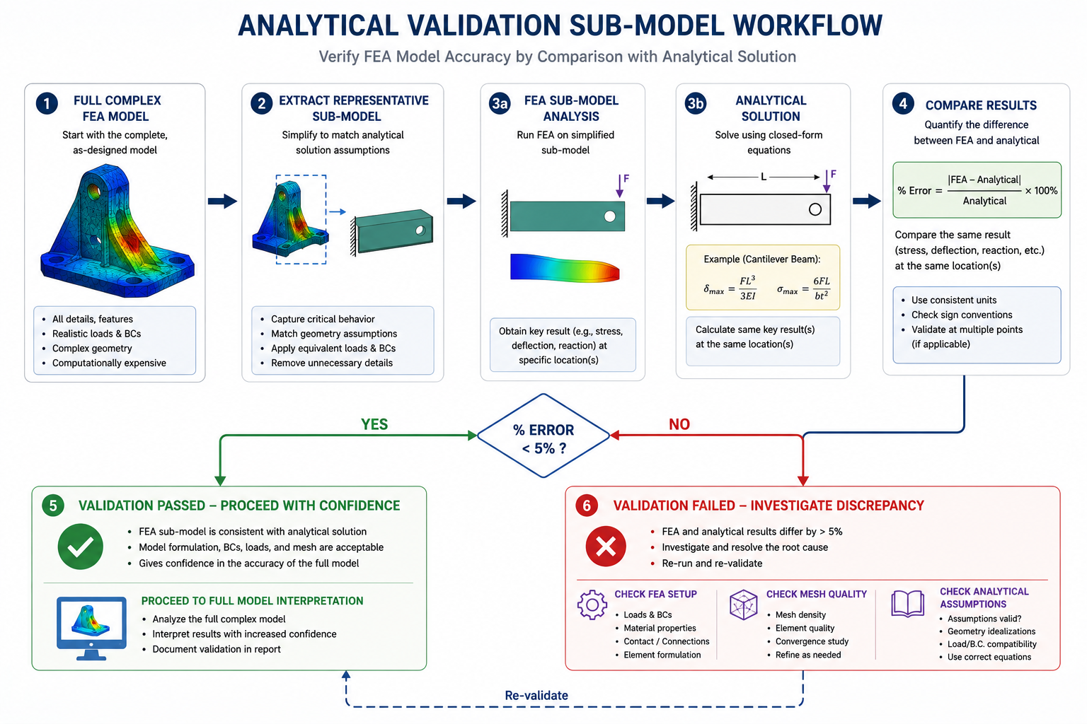
| Analytical solution comparison (Timoshenko, Roark) | Known closed-form solutions for beams, plates, cylinders, pressure vessels, confirms physics is correctly modeled | Whenever geometry can be approximated by a standard geometry with known solution | FEA result within 5% of analytical solution for the simplified geometry |
| Symmetry / antisymmetry check | Model physics is internally consistent, symmetric loads produce symmetric results, antisymmetric loads produce antisymmetric results | Any model with geometric symmetry, apply symmetric load, verify symmetric response; apply antisymmetric load, verify antisymmetric response | Stress and displacement fields mirror correctly across the symmetry plane |
| Modal analysis pre-solve check | Boundary conditions correctly remove all 6 rigid-body modes; model is properly constrained | Before every static, dynamic, or nonlinear analysis | Zero near-zero-frequency modes (all modes above 1 Hz for structural model) |
| Strain energy density check | Elements with very high strain energy density relative to neighbors may indicate mesh problems or singularities | When stress contours show isolated high-stress nodes or elements not consistent with the loading | Strain energy density should vary smoothly across the model; isolated peaks indicate mesh or BC errors |
| Physical test correlation | Complete model (physics, geometry, BCs, materials, loads) predicts measured physical test results | Whenever physical test data is available, required for model validation before results are used for design decisions | FEA prediction within 10-15% of measured strain gauge readings or 5% of measured natural frequencies at validated locations |
The Hand Calculation as the First Line of Defense
The most powerful and most underused validation tool in FEA practice is the hand calculation comparison, computing an approximate expected result using beam theory, plate theory, thin-wall pressure vessel formulas, or other closed-form methods before examining the FEA output. The hand calculation does not need to be exact: it needs to give the right order of magnitude and the right physical trend (which end deflects more, which face is in tension, where the bending moment peaks).
Before reviewing FEA results, estimate the expected stress and displacement using hand calculations. If the FEA results are within 20–30% of the estimate, the model is likely behaving correctly. Differences greater than 50% should be investigated, as they may indicate an error in the model, assumptions, or calculations that must be explained before the results are trusted.
Physical Test Correlation: The Ultimate Validation
Physical test correlation, comparing FEA predictions against measured strain gauge readings, displacement measurements, or natural frequencies from a physical prototype, is the most definitive form of simulation validation. A model that has been correlated against physical test data at multiple locations and load levels is validated; a model that has only been verified for internal consistency (reaction equilibrium, mesh convergence) is verified but not validated. The distinction matters for the confidence that can be placed in extrapolated predictions, load cases or geometric variants not covered by the physical test.
The correlation criterion: FEA predictions should agree with measured strain gauge readings within 10 to 15 percent at validated locations, and modal frequencies should agree within 5 percent for correlated natural frequencies. Discrepancies outside these ranges indicate model errors that must be identified and corrected before the model is used for design predictions. Acceptable correlation at one location does not validate the model at all locations, correlation must cover the range of stress states, boundary conditions, and geometric features that the model will be used to analyze.
The Plausibility Trap: Why Wrong Results Look Right
The defining feature of the simulation failures described in this article is that wrong results are usually plausible. The stress contours are smooth and visually credible. The deformation shape makes intuitive sense. The peak stress value is in a reasonable range, not implausibly high and not suspiciously zero. The solver completed without errors. There is nothing in the output that signals a problem to an analyst who is not specifically looking for the error class that caused it.
This plausibility is the reason systematic validation is necessary. An analyst who only reviews FEA output for plausibility, does the result look reasonable?, will miss every error that produces a plausible wrong result. This includes the physics assumption errors (linear elastic analysis of yielding material gives plausible stress distributions, just at wrong magnitudes), the boundary condition errors (fixed vs pinned gives plausible stress distributions with different values), the postprocessing errors (averaged stress at a notch gives a plausible smooth contour, just lower than the true peak), and the material model errors (wrong material data gives plausible-looking results with wrong magnitudes).
The Confirmation Bias Problem in FEA Review
FEA review is susceptible to confirmation bias in a specific and dangerous way: when the result confirms the analyst’s engineering intuition about where the highest stress should be and approximately what magnitude it should be, the review tends to stop. The result ‘makes sense,’ so it is accepted. But engineering intuition about stress magnitude is much less reliable than intuition about stress location.
An experienced engineer typically knows which feature is most highly stressed in a structure, a shoulder fillet, a bolt hole, a section transition. What engineering intuition cannot reliably predict is whether the peak stress at that feature is 185 MPa or 312 MPa, or whether it is driving a fatigue failure through von Mises or through maximum principal stress amplitude.
The protection against confirmation bias in FEA review is quantitative validation against an independent reference, not a subjective assessment of whether the result looks right. The independent reference can be a hand calculation, an analytical solution from Roark’s Formulas or Peterson’s Stress Concentration Factors, a comparison against a different FEA model with different element types or boundary condition assumptions, or a physical strain gauge measurement. Any of these provides the quantitative check that qualitative plausibility review cannot.
Building a Simulation Quality System: From Individual Checks to Organizational Process
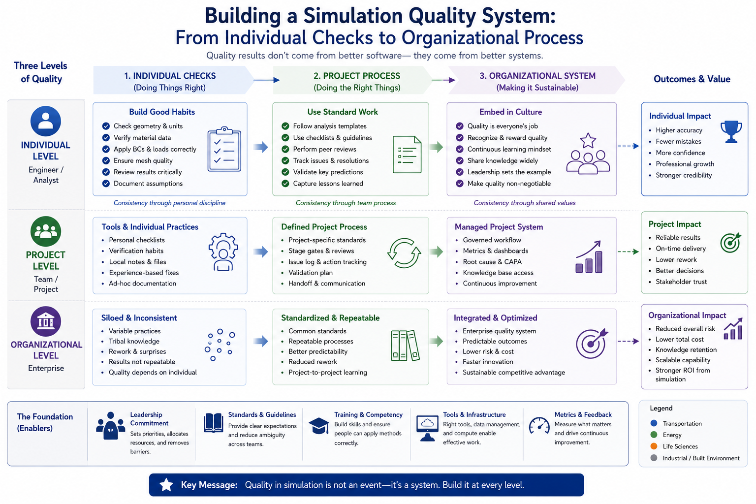
Individual analysts applying the validation methods described in this article can catch a large fraction of simulation failures. But the most effective protection against simulation failure is an organizational simulation quality system, a structured process that makes validation mandatory, creates independent review, and builds a institutional memory of the failure modes specific to the organization’s product types and analysis methods.
The Four Elements of a Simulation Quality System
- Analysis plan documentation: Before model building begins, document the analysis objective, the physics assumptions, the accepted simplifications and their justification, the load cases, the acceptance criteria, and the validation plan. An analysis plan that is reviewed before the model is built catches physics assumption errors at the lowest-cost stage, when changing the approach costs hours rather than days.
- Preprocessing checklist enforcement: The 30-point checklist from the preprocessing article in this series should be a required deliverable for every analysis, completed and signed by the analyst and reviewed by a peer. Checklist enforcement is the most efficient way to catch the preprocessing error categories: unit system inconsistency, wrong element type, missing mesh convergence studies, and boundary condition errors.
- Independent technical review: Every analysis that will be used to make a design decision or support a regulatory submission should be reviewed by an engineer who did not build the model. Independent reviewers catch assumptions that the original analyst has normalized, the BC that has always been applied this way, the material value that came from an unverified spreadsheet, the stress measure that was used in the last ten analyses without questioning its appropriateness. Peer review is the validation method with the highest return on time invested.
- Lessons-learned database: Every simulation failure that is caught, whether in internal review or by comparison with physical test data, should be documented in a format that makes it accessible to other analysts. The failure mode, the analysis type, the error category, and the detection method should all be recorded. Over time, this database becomes the organization’s institutional knowledge of which errors occur most frequently in which analysis types for which product categories, the most valuable guide to where scrutiny should be applied in future analyses.
Frequently Asked Questions
Q: If the CAD model is good and the mesh quality is good, why do FEA results fail?
FEA results can still fail because the biggest errors usually come from incorrect engineering assumptions, not the CAD model or mesh. Wrong boundary conditions, material properties, load definitions, physics selection, or failure criteria can produce inaccurate results even with a perfectly meshed model. Verification and validation are essential to detect these analyst-driven errors.
Q: What is the difference between von Mises stress and maximum principal stress, and when should I use each?
Use von Mises stress to evaluate yielding in ductile metals because it predicts permanent deformation. Use maximum principal stress for brittle materials, fatigue analysis, and fracture mechanics, where tensile stresses control failure. Choosing the wrong stress criterion can lead to incorrect safety assessments and unreliable FEA results.
Q: How do I know if a high-stress result is a real failure risk or a mesh singularity?
Refine the mesh around the high-stress region and compare the results. If the stress converges with mesh refinement, it represents a real stress concentration. If the stress keeps increasing without convergence, it is likely a mesh singularity caused by sharp corners, point loads, or idealized constraints rather than a physical failure.
Q: What is the most important validation check after running an FEA analysis?
The most important post-processing check is reaction force equilibrium. In a correct static analysis, the total reaction forces and moments should match the applied loads within an acceptable tolerance. If they do not, the model likely contains errors in boundary conditions, contacts, or load application.
Q: Can a simulation be verified but not validated, and what is the practical difference?
Yes. Verification confirms that the mathematical model has been solved correctly, while validation confirms that the model accurately represents the real physical system. A simulation can be numerically correct but still produce misleading results if the underlying assumptions, materials, or boundary conditions do not reflect reality.
Q: What is the most dangerous simulation failure mode, the one most likely to cause a real-world product failure?
The most dangerous failure mode is a non-conservative simulation, where the model predicts a design is safe when it is not. This often results from incorrect boundary conditions, inappropriate physics assumptions, or using the wrong failure criterion, leading to unsafe engineering decisions despite apparently acceptable FEA results.
Conclusion:
The message of this article can be stated directly: simulation fails because of decisions the analyst makes, not because of the quality of the CAD model. CAD geometry is the starting point for FEA, but it is not the determinant of FEA accuracy. The determinant is the quality of the judgments made at every step from physics selection to results interpretation, judgments that the software cannot make, the mesh cannot correct, and the solver cannot verify.
The twelve failure categories in this article, from wrong physics assumptions through postprocessing interpretation errors, share a common feature: they are all analyst decisions. They are decisions about which equations to solve, which material behavior to assume, how to represent supports and loads, and how to read the output. Improving these decisions requires not better software or better CAD, but better physics understanding, more rigorous validation habits, and organizational processes that make systematic review the default rather than the exception.
The practical implication for any engineering organization that uses FEA: the return on investment from analyst training and validation process improvement exceeds the return from higher-end simulation software, better hardware, or higher-quality CAD tools, because the errors that training and process improvement address are the dominant sources of wrong results. A well-trained analyst with rigorous validation habits using mid-tier software produces more reliable results than an untrained analyst with premium tools and perfect CAD. The tools serve the judgment. The judgment is what determines whether the simulation is worth trusting.
Strengthen your simulation practice with our guides on FEA preprocessing, boundary condition selection, static vs dynamic analysis, stress concentration, mesh quality, and the top industries where simulation accuracy determines product success.