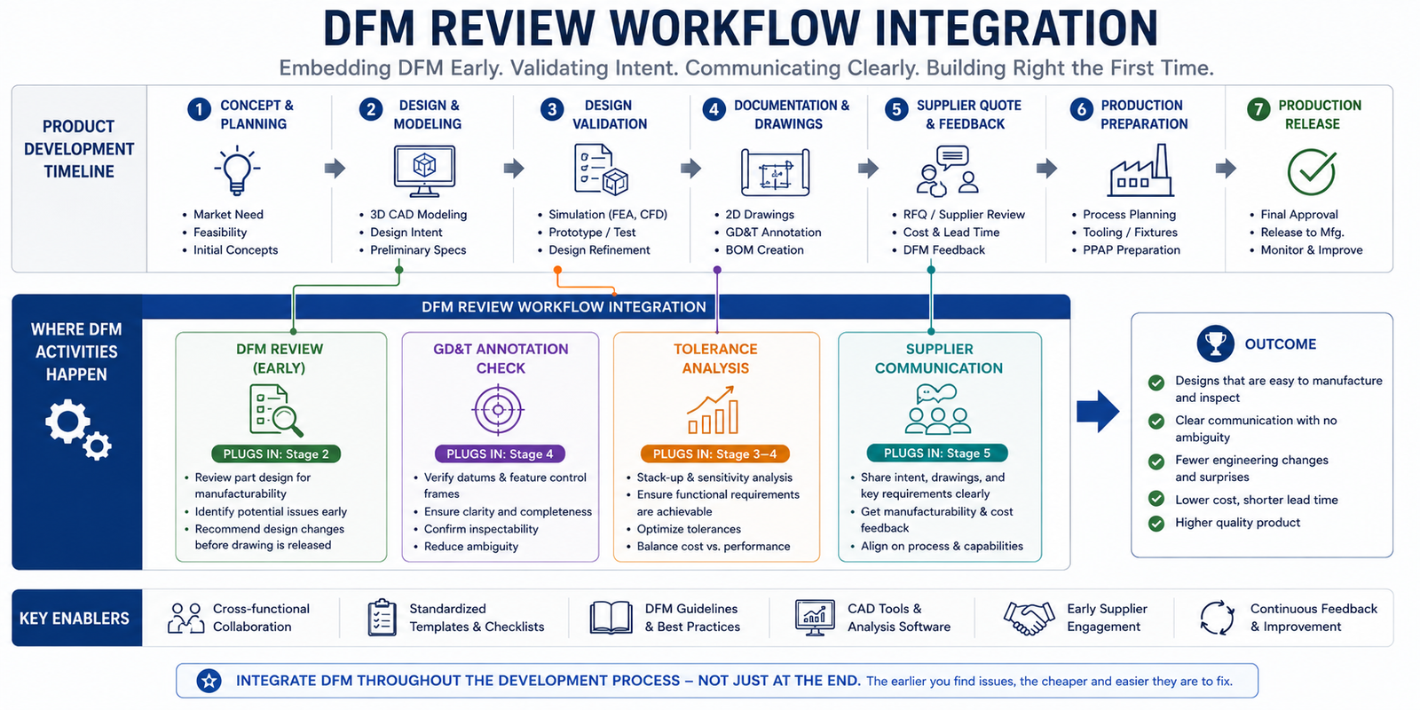
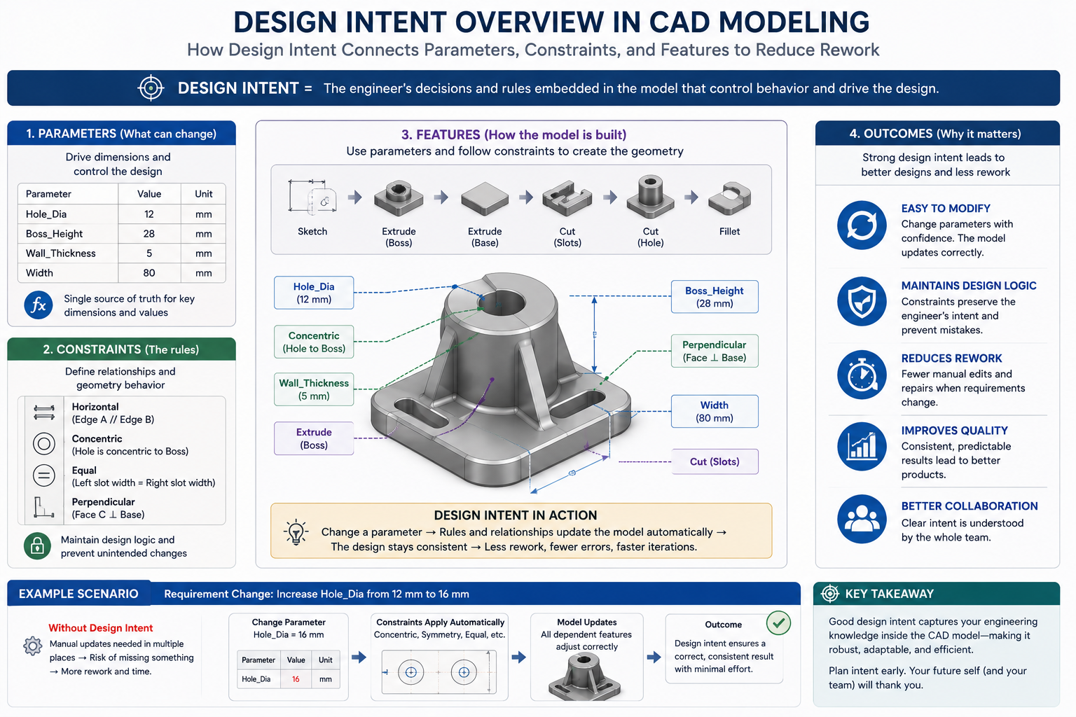
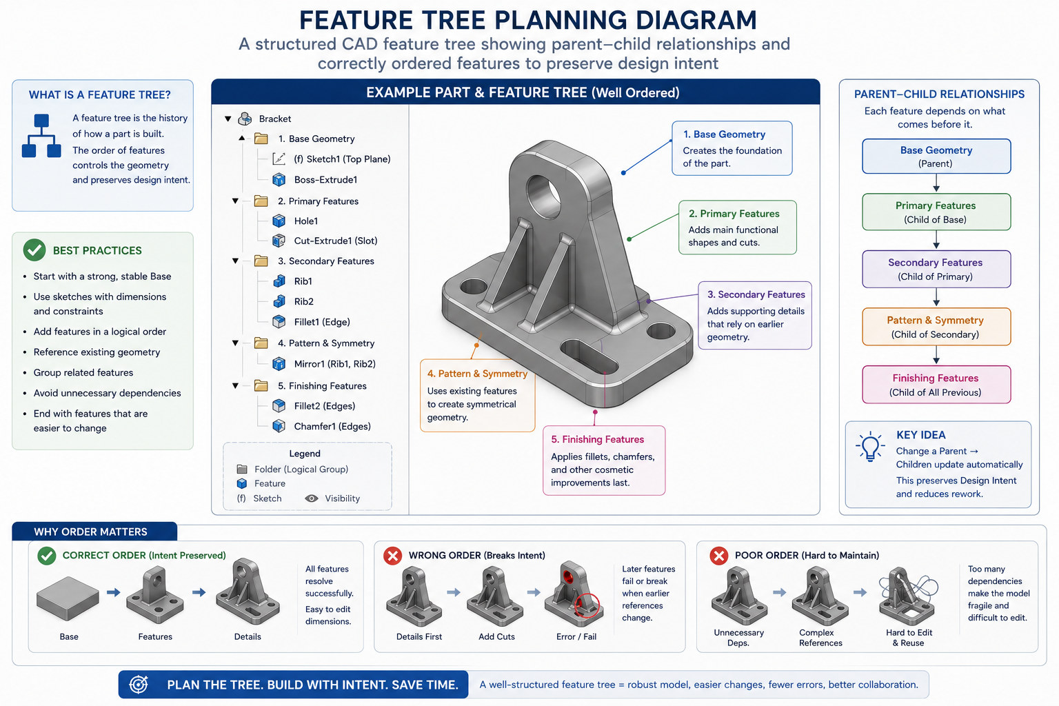
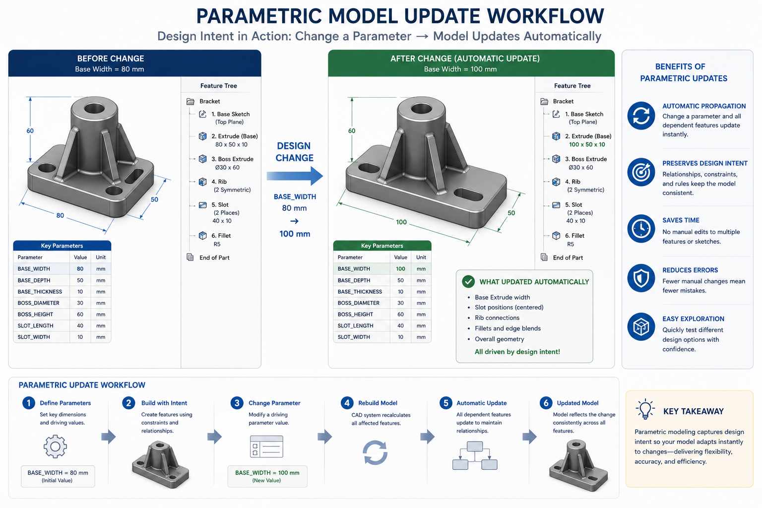
If you’re still manually rebuilding 3D models from old 2D drawings, you’re spending hours on work that modern tools can now do in minutes. Automating 2D to 3D CAD conversion for CNC machining means using software, rather than a person at a keyboard, to turn a flat drawing into a solid model a CAM program can actually machine from.
QUICK ANSWER Yes, you can automate 2D to 3D CAD conversion using one of four methods: native CAD conversion wizards, dedicated conversion software, AI-based reconstruction, or custom API scripting. For CNC machining specifically, the output needs to be a true parametric STEP solid, not just a visual mesh, and it should always be checked for dimensional accuracy before it goes to CAM.
This guide covers all four automation methods side by side, which file format actually works for CNC, how accurate automated conversion really is, and a step-by-step process to get from a flat drawing to a CNC-ready 3D model without wasting a machining run on a bad file.
What Does It Mean to Automate 2D to 3D CAD Conversion?
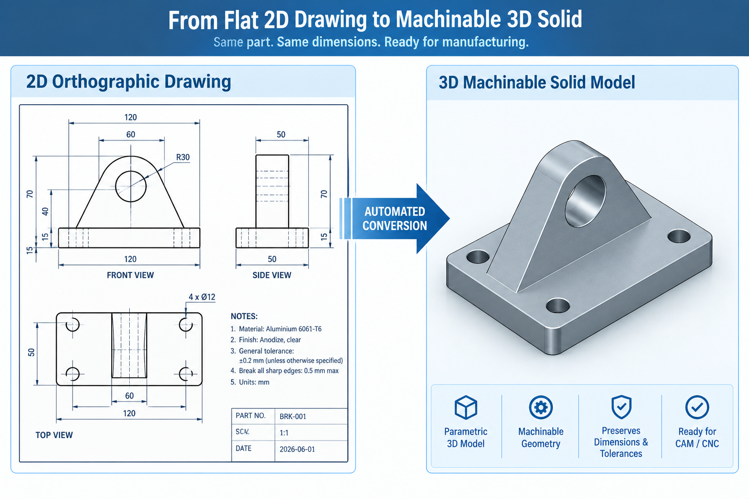
Automating 2D to 3D CAD conversion means letting software interpret a 2D drawing’s lines, arcs, and dimensions, and reconstruct it as a three-dimensional solid, without an engineer manually redrawing every feature by hand.
This matters specifically for CNC machining because CAM software doesn’t cut from a 2D drawing. It needs a 3D solid model to calculate toolpaths, cutter clearances, and machining operations. If your only source is an old drawing, a scanned PDF, or a customer sketch, automated conversion is what bridges that gap without a full manual rebuild.
4 Ways to Automate 2D to 3D CAD Conversion
There isn’t one single tool that does this for everyone. The right method depends on your drawing volume, your budget, and how much accuracy you need. Here are the four real approaches used in production today.
Automation Method
How It Works
Best For
Main Limitation
Native CAD conversion tools
Built-in wizards inside SolidWorks, Autodesk Inventor, Fusion 360, and Siemens NX that read a 2D DXF/DWG sketch and extrude, revolve, or auto-sequence it into a solid model
Teams already standardized on one CAD platform who need a fast, in-house way to rebuild simple to moderately complex parts
Struggles with parts that have implied features (fillets, complex holes) not explicitly drawn on every view
Dedicated CAD conversion software
Standalone tools such as Scan2CAD or Aspose.CAD that specialize in reading raster images, PDFs, or scanned drawings and outputting clean, editable vector or solid geometry, often with batch and API automation
Digitizing large archives of legacy paper drawings or scanned PDFs at scale, especially for spare-parts and MRO workflows
Output is typically a clean 2D vector file or basic solid, still needs review before it’s treated as production CAD
AI and deep-learning reconstruction
Machine learning models trained to recognize geometric features across multiple 2D views (or even photos) and infer a 3D shape, an active and fast-moving research area as well as a growing commercial category
Fast first-pass geometry when the original CAD file is lost but a drawing, PDF, or photo still exists, and speed matters more than final precision
Output is usually a mesh or an unverified solid: no GD&T, no material data, and dimensions that must be checked before machining
Scripting and API-driven automation
Custom scripts built on CAD APIs (NX Open, SolidWorks macros, Fusion 360’s Python API) that batch-process large sets of similar 2D drawings into 3D models using a repeatable, rule-based logic
Manufacturers with high volumes of similar, well-standardized drawings, such as a family of brackets or fasteners, where the same rules apply every time
Requires upfront engineering investment to build and maintain the script; not cost-effective for one-off or highly varied parts
Feature Recognition vs. AI Mesh Generation: Know the Difference
This is the distinction most articles on this topic skip, and it’s the one that actually matters most. Feature recognition (used by native CAD tools and dedicated conversion software) analyzes geometric intent, holes, pockets, fillets, and rebuilds them as true, editable, dimensioned solid features.
AI mesh generation (used by many newer AI tools) predicts an approximate 3D shape from limited 2D input. The result often looks convincing on screen, but it’s typically a mesh with no feature history, no tolerances, and no guarantee the dimensions match the original drawing exactly. Recent peer-reviewed research on deep-learning-based reconstruction confirms this gap is a structural limitation of current methods, not just a rough edge that will disappear with the next software update (more on that in the accuracy section below).
Which File Format Actually Works for CNC Machining?
Automation only helps if the output file is something your CAM software can actually use. Here’s how the common formats stack up.
File Format
Geometry Type
Good for CNC Machining?
Why
STEP (.step/.stp)
True parametric/B-rep solid
Yes , the standard choice
Preserves exact solid geometry that CAM software can read directly for toolpath generation
DXF/DWG
2D vector lines and arcs
Only for 2D profile cutting
Fine for laser, waterjet, or simple 2D milling; not a 3D solid on its own
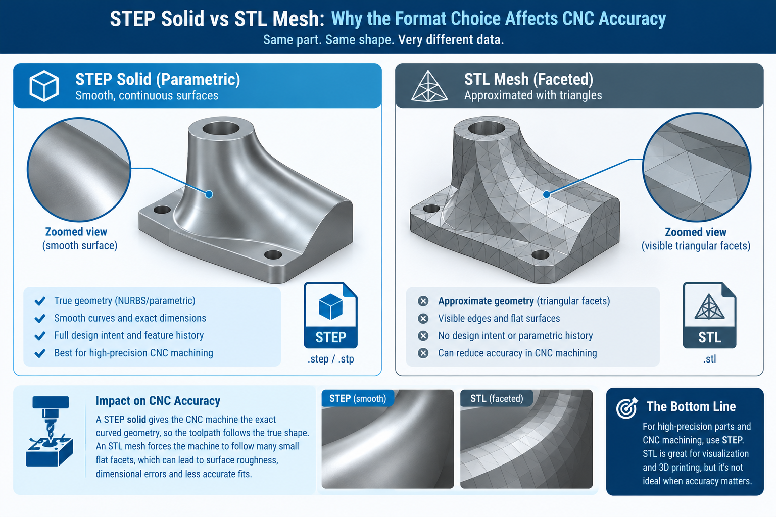
STL
Triangulated mesh (approximation)
Not recommended for milling
Approximates curved surfaces with flat facets, which can introduce dimensional error on tight-tolerance features
IGES (.igs)
Surface/solid model
Usable, but aging
Still supported by most CAM systems, though STEP has largely replaced it as the preferred neutral format
If a conversion tool only offers STL output, treat it as a visualization step, not a finished CNC-ready file. For milled or turned parts, always push for a STEP solid before it goes anywhere near a CAM program.
Step-by-Step: From 2D Drawing to CNC-Ready 3D Model
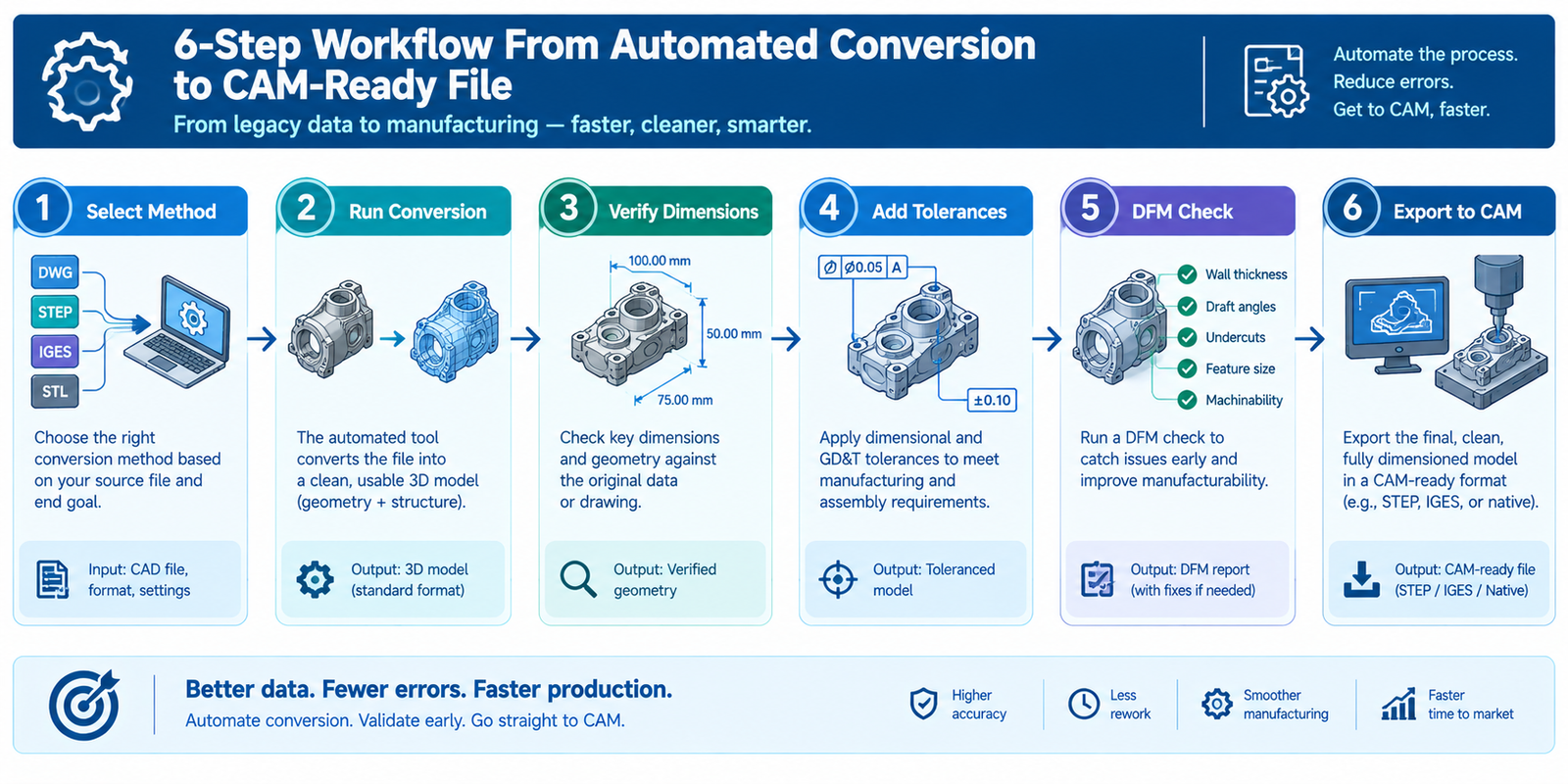
Choose the right automation method: match the method to your situation using the table above, don’t default to whatever tool you already own if it’s the wrong fit for the job.
Run the automated conversion: feed in the cleanest source file available, native DXF/DWG beats a scanned PDF, and a scanned PDF beats a blurry photo.
Verify every critical dimension: cross-check the converted model’s key dimensions against the original drawing before trusting it, especially on mating features and hole positions.
Add tolerances and GD&T: automated conversion rarely carries tolerance information forward, so this has to be added manually to define acceptable variation for the machinist.
Run a design-for-manufacturability (DFM) check: confirm the geometry is actually machinable, watch for internal corners, deep pockets, and wall thicknesses your specific CNC setup can’t reliably hold.
Export to STEP and import into CAM: generate toolpaths only once the solid model has passed the checks above, not directly from the raw conversion output.
How Accurate Is Automated 2D-to-3D Conversion, Really?
Accuracy depends entirely on the method and the source drawing quality. Native feature-recognition tools working from a complete, well-dimensioned DXF file can rebuild simple to moderately complex parts with very high fidelity, because they’re following explicit geometric rules, not guessing.
AI-based reconstruction is a different story. It’s genuinely useful for getting a fast first-pass shape when the original CAD file is gone and only a drawing or photo survives, but current research is clear that the output should be treated as a reference model, not production-ready CNC data, until an engineer verifies it. A 2026 peer-reviewed study on deep-learning-based 2D-to-3D conversion found that combining automated feature recognition with structured verification meaningfully reduced dimensional errors compared to AI inference alone, reinforcing that human review is still the difference between a usable model and a expensive machining mistake.
Common Mistakes to Avoid
Sending an STL straight to CAM: meshes approximate curves with flat facets, which can create real dimensional error on toleranced features.
Trusting AI-generated geometry without verification: a visually convincing model is not the same as a dimensionally accurate one.
Skipping GD&T entirely: without tolerance information, a machinist has no way to know what deviation is actually acceptable.
Using one tool for every job: a batch-scripting solution built for a family of brackets won’t serve you well for a single, highly custom part, and vice versa.
Assuming automation removes the need for review: automation speeds up the first draft; it doesn’t replace an engineer’s final check.
Frequently Asked Questions
Q: Can AI convert a 2D drawing into a CNC-ready 3D model?
AI can generate a 3D shape from a 2D drawing quickly, but the output is usually a mesh that needs dimensional verification before it’s safe to machine from. Treat it as a fast first draft, not a finished CNC file.
Q: What is the best file format for CAD to CNC conversion?
STEP is the best format for CNC milling and turning because it preserves true, editable solid geometry. STL is fine for 3D printing but can introduce dimensional error on machined parts.
Q: How accurate is automated 2D-to-3D CAD conversion?
Rule-based feature recognition from a clean, complete drawing is typically very accurate. AI-based reconstruction is faster but less reliable and should always be verified against the original dimensions before use.
Q: What software automatically converts 2D CAD drawings to 3D models?
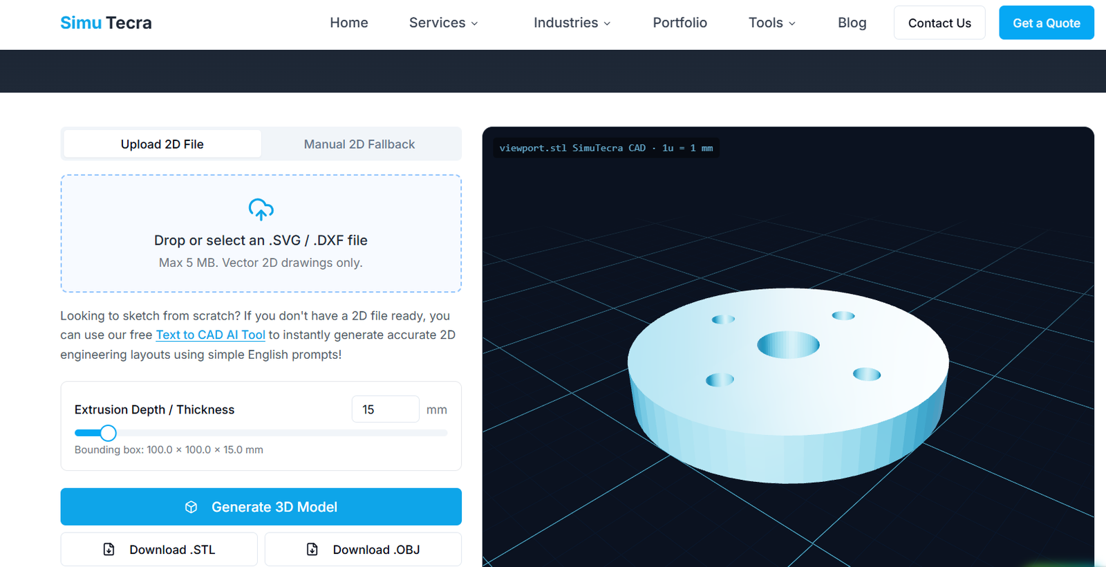
Simutecra 2D CAD to 3D CAD, SolidWorks, Autodesk Inventor, and Fusion 360 include built-in conversion tools, while Scan2CAD and similar dedicated software specialize in converting scanned or legacy 2D drawings at scale.
Q: Do I still need an engineer to review an automatically converted 3D model?
Yes. Automation speeds up the initial rebuild, but dimension verification, tolerance assignment, and a manufacturability check still require engineering review before the file goes to CAM.
Conclusion
Automating 2D to 3D CAD conversion for CNC machining can save real time, but only if you match the method to the job and never skip verification. Use native or dedicated feature-recognition tools when accuracy matters most, reach for AI reconstruction when speed matters more than precision and the file can be reviewed afterward, and always export a true STEP solid, with tolerances added, before it reaches your CAM software.
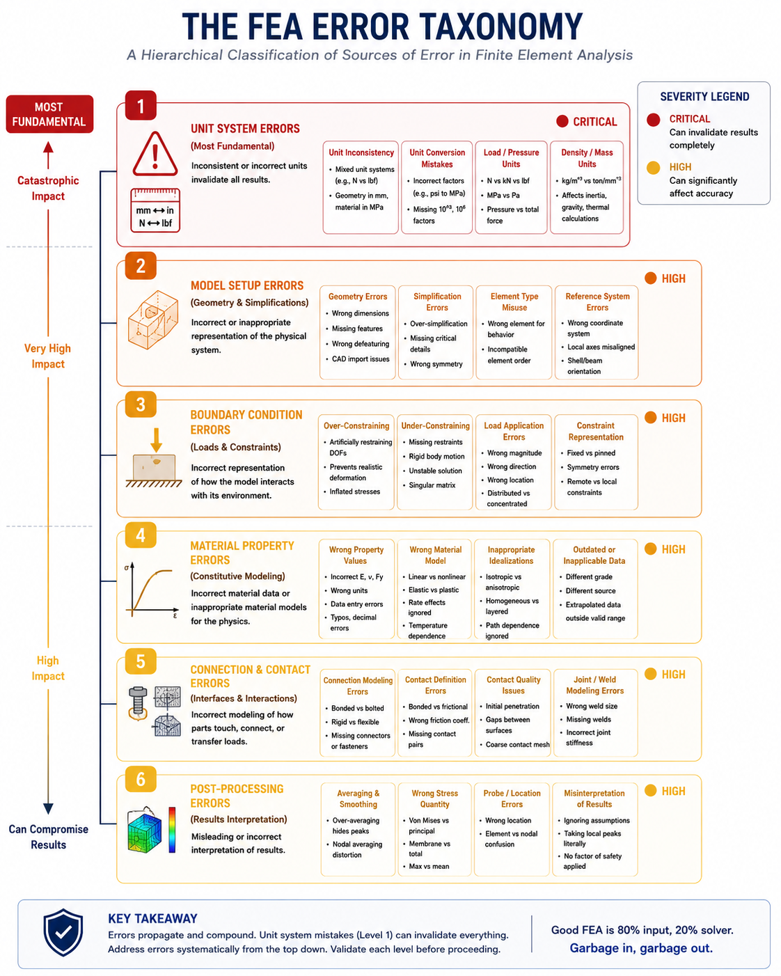
The FEA model runs. The solver converges without warnings. The results are presented to the design team, the safety factor looks adequate, and the design is approved. Six months later, during testing or worse, during service, something fails in a way that the analysis did not predict. The investigation that follows invariably finds one or more of the same categories of error that appear in this article, committed during the analysis phase and not detected before the decision was made.
What makes FEA errors particularly dangerous is not that they are hard to understand once identified. It is that many of them produce results that look entirely plausible. The stress contour map has smooth gradients. The deformed shape looks reasonable. The solver did not report any errors or warnings. The peak stress is in a location that makes intuitive sense. The only problem is that the actual stress is three times higher, or the failure mode is entirely different, or the model is six times stiffer than reality because of an over-constraining boundary condition that was never questioned.
This article covers 16 specific FEA errors organized into six categories, each explained with the root cause that produces it, the magnitude and type of result error it causes, and the specific detection method that will catch it before it leads to a wrong engineering decision. The goal is not just to document mistakes but to give engineers the diagnostic toolkit to find and correct them systematically.
Error Overview: 16 Mistakes Mapped to Impact and Detection
The following table maps all 16 errors covered in this article to their typical result impact, detection method, and severity. Use it as a quick reference during model review, and refer to the detailed sections for each error category for the full technical explanation.
Error Category
Specific Error
Typical Impact on Results
Detection Method
Severity
Unit system
Mixing mm and m, N and kN in same model
Factor of 1000 to 1,000,000 error on stresses
Reaction force check vs expected; dimensional sanity check
Critical – always catastrophic
Boundary conditions
Over-constraining with fixed wall instead of pin
50-500% stiffness overestimation in bending
Deformation mode review; compare reaction moments vs applied
High – systematic error
Boundary conditions
Under-constraining – rigid body motion
Solver failure or near-singular matrix
Modal analysis with 6 zero-frequency modes expected
Critical – analysis is invalid
Boundary conditions
Artificial stiffness from enforced displacement on unintended DOF
Local stress artifacts near constraint; global stiffness wrong
Remove constraint and observe deformation change
High
Material properties
Wrong Young’s modulus (10x too high/low)
Displacements off by 10x; stress unchanged if load-controlled
Verify against published data; check material units
High
Material properties
Linear material used beyond yield
Predicted stress above Sy with no yielding shown
Check peak von Mises vs Sy; run with elastoplastic model
Very High – unsafe
Material properties
Unit system error in material (GPa vs MPa)
1000x error on stress; displacement changes by 1000x
Sanity check displacement magnitude vs expected
Critical
Connection
Bonded instead of frictional contact
Artificially high force transfer; no sliding captured
Check contact pressure distribution; sliding in physical test?
High
Connection
Disconnected mesh nodes at part interface
Load not transferred; stress concentration at gap
Plot deformed shape; check force transfer through interface
Critical – load path wrong
Mesh
Coarse mesh at stress concentration
Peak stress underestimated by 50-90%
Mesh convergence study at concentration
High
Mesh
Linear tet in bending-dominated region
Bending stiffness 2-5x too high; stress wrong
Switch to quadratic tet; re-run and compare
High
Loads
Wrong load direction (global vs local coordinates)
Completely wrong deformation mode
Deformation mode check; verify against expected
Critical – completely wrong
Loads
Load magnitude in wrong unit (N vs kN)
1000x error on all stresses
Equilibrium check; compare reaction to applied
Critical
Analysis type
Linear used for geometric nonlinear problem
Stiffness wrong; snap-through missed
Check displacement/dimension ratio; run NL and compare
High
Post-processing
Reading averaged instead of unaveraged stress
Peak stress artificially reduced by averaging
Switch to unaveraged; check gradient across element
High – masks failure risk
Post-processing
Von Mises instead of principal for brittle failure
Wrong failure criterion applied
Check failure mode; use max principal for brittle
High
The severity classification reflects the potential for the error to lead to an engineering decision that would be different if the model were correct. Critical errors produce results so wrong that no engineering decision made from them should be trusted. High errors produce systematically biased results that may lead to unconservative or over-conservative decisions. The most dangerous errors are those that produce plausible-looking results that do not trigger the analyst’s suspicion.
Error Category 1: Unit System Inconsistency
Unit system errors are the most catastrophically damaging FEA mistakes because they produce errors by factors of 1,000, 1,000,000, or more, in results that look entirely reasonable in magnitude because the analyst has no independent reference for what the correct answer should be. A unit system error is a silent multiplier that scales every result in the model by a constant factor without triggering any solver warning, any convergence issue, or any plausibility check that is not deliberately applied by the analyst.
How Unit System Errors Happen
FEA solvers do not have a built-in unit system. They process numbers. The solver does not know whether the number 210,000 you entered as Young’s modulus represents 210,000 MPa (correct for steel in MPa units) or 210,000 Pa (steel modulus 1,000,000 times too low) or 210,000 GPa (steel modulus 1,000 times too high). The solver accepts whatever numbers you provide and produces results in the same unit system those numbers imply. If you enter modulus in MPa, forces in N, and geometry in mm, the solver returns stresses in MPa and displacements in mm. If you mix these units, the results are in whatever undefined mixed unit system your inputs created.
The most common mixing error: geometry imported from a CAD system in millimeters, forces applied in kilonewtons (as copied from a load specification), and Young’s modulus entered in GPa (from a materials datasheet that uses GPa). The solver receives: geometry in mm, forces in kN, modulus in GPa. It computes stresses in GPa·kN/mm^2, which is not a standard unit, and the result is numerically somewhere between 10^3 and 10^6 times the correct stress value depending on the specific combination. The displacement result has the same problem. The contour plot still looks smooth and plausible because the color scale adjusts to whatever range the results happen to cover.
The Detection Method: Four Mandatory Unit Checks
Consistent unit table before any model is started: write out your unit system explicitly before beginning. For SI: force in N, length in m, stress in Pa. For SI-mm: force in N, length in mm, stress in MPa. For US customary: force in lbf, length in in, stress in psi. Every input to the model must be in this system.
Dimensional sanity check on displacements: run a quick estimate of the expected displacement before reviewing FEA results. A steel cantilever beam 200mm long, 10mm square, loaded with 10N at the tip should deflect approximately 5mm by beam theory. If your FEA shows 0.005mm or 5000mm, you have a unit error.
Equilibrium check on reactions: the reaction forces at your boundary conditions must sum to the applied loads. If you applied 1000N and the solver reports a 1.0N reaction, your forces are in kN but you entered them expecting N.
Stress sanity check: the peak stress should be in a physically plausible range. For steel with 10N applied to a 10mm square bar (cross-section area 100mm^2), the nominal stress is 0.1 MPa. If your FEA shows 100 GPa, there is a unit error in the material or load.
Unit System Reference Card SI-mm (most common for mechanical engineering): Length: mm | Force: N | Mass: tonne (1000 kg) | Time: s | Stress: MPa (N/mm^2) | Modulus: MPa | Density: tonne/mm^3 (steel: 7.85e-9) | Thermal: mm, C, W/mm.C. SI (structures/civil): Length: m | Force: N or kN | Stress: Pa or kPa | Modulus: Pa or GPa. CRITICAL: never mix mm-geometry with GPa-modulus without explicitly converting. Steel modulus in SI-mm units = 210,000 MPa, NOT 210 GPa.
Error Category 2: Boundary Condition Errors
Boundary condition errors are the most consequential modeling mistakes for structural accuracy. The boundary conditions define how the structure is supported and loaded, and an incorrect constraint fundamentally changes the structural problem being solved. No amount of mesh refinement or solver sophistication can correct for a boundary condition that does not represent the physical support condition. The mesh quality article in this series can be thought of as optimizing the numerical solution to a mathematical problem; boundary condition errors change the mathematical problem itself.
Over-Constraining: Adding Stiffness That Does Not Exist
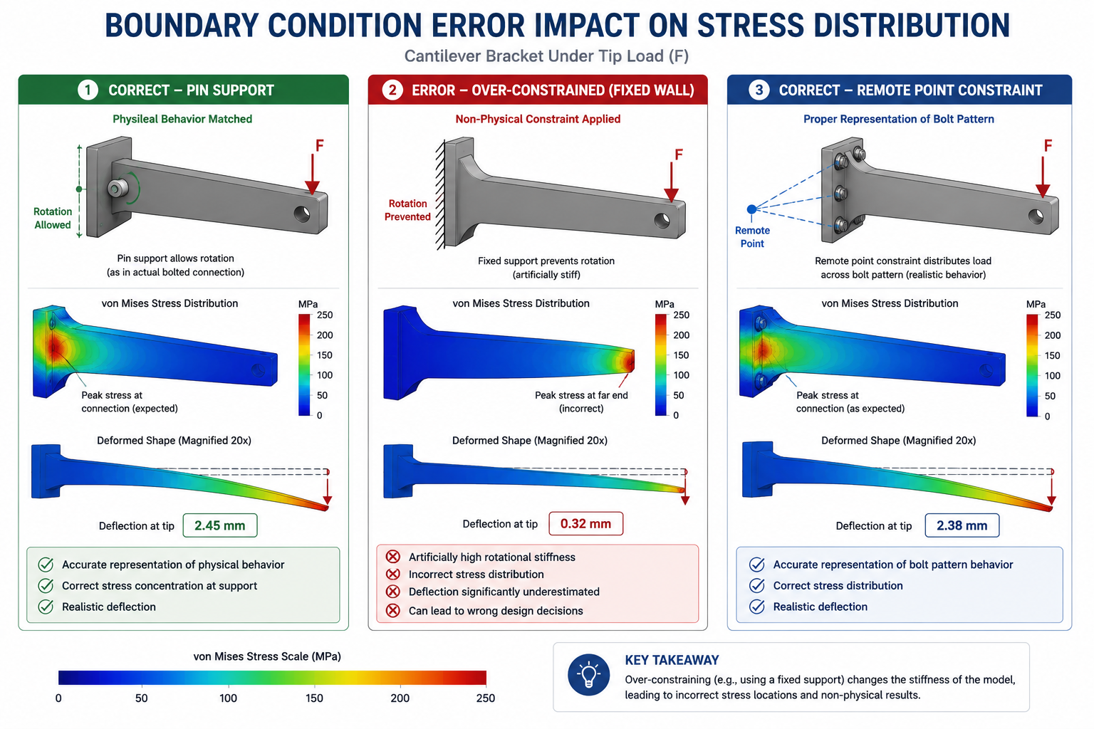
The most common boundary condition error in structural FEA is over-constraining: applying more constraint than the physical support actually provides. The classic example is using a fixed wall (all six degrees of freedom constrained: three translations and three rotations) to represent a bolted connection where the bolts provide translational constraint but do not prevent rotation. The fixed constraint provides infinite rotational stiffness at the connection. The real bolted joint provides finite (and often low) rotational stiffness. The result: the FEA model is systematically stiffer than the real structure, producing lower deflections and potentially lower peak bending stresses than will exist in the physical part.
The quantitative impact of over-constraining depends on the structural geometry but can be substantial. For a cantilever beam of moderate slenderness ratio (length/height approximately 10:1), replacing a pin support (translational constraint, no rotational constraint) with a fixed support (full constraint) increases the structural stiffness by approximately 4 times and reduces the tip deflection by 4 times for the same applied load. The peak stress location also shifts from the constraint location to the mid-span in some load cases. A design decision made on fixed-support FEA results for a pin-supported real structure may be unconservative by this factor.
Under-Constraining: Rigid Body Motion
The opposite error, under-constraining, produces an ill-conditioned or singular stiffness matrix that the solver cannot invert. The symptom is either a solver error (negative pivot, singular matrix, rigid body motion detected) or, in some solvers with soft springs for stabilization enabled by default, extremely large displacements that indicate unconstrained motion. Under-constraining typically happens when a model is intended to be symmetric but the symmetry boundary conditions are not correctly applied, when a part is connected to adjacent structure through contact only and the contact has not yet engaged, or when the analyst is modeling a sub-structure and has not fully defined the interface with the surrounding structure.
Detection is straightforward: run a modal analysis (natural frequency extraction) on the model before the static analysis. An unconstrained model will show six rigid body modes at or near zero frequency (three translations and three rotations with zero elastic stiffness). Each unconstrained DOF in the model corresponds to one zero-frequency mode. The mode shapes of the zero-frequency modes directly identify which translations and rotations are unconstrained, pointing to the specific missing boundary conditions.
Artificial Stiffness from Constraint Location and Type
A subtler constraint error that produces locally incorrect results without making the global analysis obviously wrong is applying displacement constraints directly to mesh nodes that are on or adjacent to the region of engineering interest. A fully fixed node creates a stress concentration artifact at the constraint location that is entirely a modeling artifact, not a real physical feature. The reported stress at and near the fixed node is meaningless, and if the stress concentration from the constraint overlaps with the real stress concentration from the geometry, the analyst cannot easily separate the physical and artificial contributions to the peak stress.
The correct approach for any support condition that is not literally a fully fixed rigid wall is to apply constraints through remote points, rigid elements, or multi-point constraints (MPC) that distribute the constraint over a realistic contact area, or to replace the support with a spring element calibrated to the actual support stiffness. This separates the constraint mechanism from the geometry of interest and prevents the artificial stress concentration artifact at the constraint location.
Boundary Condition Best Practice Before applying any constraint, ask: What physical mechanism provides this support in the real structure? A bolted joint provides translational stiffness and partial rotational stiffness, not infinite rotational stiffness. A bearing provides radial stiffness but typically not axial or moment stiffness unless specifically designed to do so. A weld provides all six DOF. Model the mechanism, not the assumption. When in doubt about the rotational stiffness: run the analysis twice, once with all six DOF fixed and once with only translational DOF fixed (pin-equivalent). The true answer lies between these bounds, and if they differ significantly, the rotational stiffness assumption is important and needs investigation.
Error Category 3: Material Property Errors
Material property errors are the category that most consistently surprises analysts because FEA software makes entering material properties feel authoritative: you type a number, the software accepts it, and the model runs. The software has no way to know whether the number you entered is correct for your material, in your unit system, at the relevant temperature, in the relevant manufacturing condition. Material property errors are therefore entirely the analyst’s responsibility to detect, and they can remain undetected through mesh convergence studies, equilibrium checks, and deformation mode reviews because these validation steps do not require correct material properties to pass.
Wrong Young’s Modulus: The Invisible Stiffness Error
An incorrect Young’s modulus shifts every displacement and stress in a load-controlled analysis by the ratio of the wrong modulus to the correct modulus. Using 210,000 Pa instead of 210,000 MPa for steel (a factor of 1,000,000 error from GPa-to-Pa confusion) produces displacements 1,000,000 times too large and reactions and stresses that appear incorrect because the structure is effectively compliant rubber rather than steel. This extreme case would be immediately obvious from a displacement sanity check.
More insidious: using 70,000 MPa (aluminum modulus) instead of 210,000 MPa (steel modulus) in a steel component, perhaps because the analyst copied material data from a previous aluminum project. The model runs correctly in every formal sense. Displacements are 3x too high (aluminum is 3x less stiff). Stresses, for a load-controlled analysis, are unchanged (stress = load/area, independent of modulus for statically determinate structures) but deflections affect the load path in statically indeterminate structures. The deformed shape looks qualitatively correct. Only a quantitative check against a hand calculation for the specific deflection catches this error.
Linear Material Beyond Yield: The Most Dangerous Material Error
Using a linear elastic material model in a situation where the true material behavior is elastoplastic is the single most dangerous material error in structural FEA because it produces results that appear to show an adequate safety factor when the real structure has actually yielded and may be near plastic collapse. A linear elastic model reports that the stress at a location is 450 MPa on a steel with a yield strength of 250 MPa. This is a physically impossible result: the real material cannot sustain 450 MPa elastically. But the solver has no knowledge of the yield strength and reports the linear elastic result without comment.
The analyst who reads 450 MPa from a linear elastic model on a 250 MPa yield-strength steel must recognize that the result cannot be the true stress. The real stress is bounded by the yield strength (in the absence of strain hardening), and the real strain is much larger than the linear analysis predicts because the material is yielding and absorbing energy that the linear model assumes is being stored elastically. For a safety assessment, any linear elastic FEA result exceeding the yield strength must be flagged and either investigated with an elastoplastic analysis or assessed using plasticity correction methods (Neuber’s rule, ESED method) specifically developed for this situation.
Temperature-Dependent Properties at Wrong Temperature
Many materials show significant changes in mechanical properties with temperature: Young’s modulus decreases, yield strength decreases, creep rate increases. An FEA analysis using room-temperature material properties for a component operating at 400 to 600 degrees Celsius, a typical turbine blade or exhaust manifold operating condition, may overestimate stiffness by 20 to 40 percent and overestimate yield strength by 50 to 70 percent compared to the actual elevated-temperature properties. The resulting safety factor is fictitious: it reflects the room-temperature material, not the material at operating temperature.
Detection requires knowing the operating temperature and verifying that the material properties in the model match published data at that temperature, not at room temperature. For thermal-structural coupled analyses, the temperature field must be correctly computed and the temperature-dependent material properties must be defined as functions of temperature in the material model, not as single values at one temperature.
Error Category 4: Connection and Contact Errors
In multi-body assemblies, the connection between parts is a modeling decision with direct consequences for load transfer, stress distribution, and overall structural stiffness. A wrong contact assumption is often worse than no contact at all, because it creates a plausible-looking stress distribution that silently transfers load in the wrong way. The most common FEA software defaults to bonded contact for all contact pairs, which means that unless the analyst explicitly changes the contact type, every touching surface in the model is assumed to be rigidly glued to every other touching surface.
Bonded Contact: When It Applies and When It Does Not
Bonded contact treats two surfaces as if they are welded or adhesively bonded with no possibility of separation, sliding, or relative displacement. It is appropriate for: welded connections (if the weld is not being analyzed for integrity), adhesive bonds that will not be stressed beyond their elastic limit, and press-fit interfaces where the contact pressure is sufficient to prevent any relative motion. It is not appropriate for: bolted connections (which can open under tension and slide under shear if the friction is overcome), bearing contacts (which can separate), snap-fit connections (which can disengage), and any interface where the contact state might change during loading.
The specific error from using bonded contact where frictionless or frictional contact is correct: the bonded interface transmits tensile force across the contact faces, which is physically impossible for surfaces that are merely in contact without adhesion. This results in artificially high load transfer across what should be a compression-only interface, changing the stress distribution in both parts and potentially masking a separation condition that would create a stress concentration in the physical assembly that the bonded model never shows.
Disconnected Mesh Nodes: The Silent Load Path Failure
In an assembly model where parts are meshed independently and then positioned in contact, it is possible for mesh nodes at the interface to be very close to each other but not actually connected. If the solver does not detect a contact pair between the surfaces (because the contact definition was omitted or the contact detection tolerance is not set wide enough to find the gap), the model treats the two surfaces as if they are in free air. No load transfers between them.
This error is particularly insidious because the model runs without error, the convergence is good, and the deformed shape may look physically reasonable on the non-loaded side. The error appears as one part moving through another in the deformed shape (interpenetration) or as a complete absence of stress in the part that should be receiving load through the contact interface. Detection: plot the deformed shape with the actual scale factor (1:1, not exaggerated) and look for interpenetration. Check that the force transferred through every interface equals the expected proportion of the applied load.
Error Category 5: Load Application Errors
Load application errors cause the analysis to solve the wrong physical problem. Unlike material errors, which affect the magnitude of results while leaving the qualitative pattern correct, load direction errors can produce a completely different deformation mode and stress distribution from the physically correct solution. A structure loaded in the Z-direction that is analyzed with the load in the X-direction (perhaps because global coordinate axes were confused with local component axes) will show maximum stress in the wrong member, maximum deflection in the wrong direction, and completely wrong reactions.
Load Direction Errors: Global vs Local Coordinates
The most common load direction error is applying a load in the global coordinate system direction when it should be in a local coordinate system direction, or vice versa. Gravity, for example, acts in the global Y (or Z, depending on the model orientation) direction. A component that is angled at 30 degrees to horizontal has gravity acting along that angle in global coordinates, but if the analyst applies gravity as a vertical downward force in global coordinates and the model is oriented with the component vertical in the model space, the load is applied in the wrong direction relative to the component geometry.
The detection method is the deformation mode check: review the deformed shape and ask whether the structure deflects in the direction you would expect given the applied load direction. If the deformation is perpendicular to the expected direction or shows a mode that does not match the loading, a load direction error is the likely cause. For models with distributed pressure loads, plot the load direction vectors as arrows on the model surface and verify they are pointing in the correct direction relative to the geometry.
Pressure Load on Wrong Surface Orientation
Surface pressure loads in FEA are applied normal to the surface element face. The direction of this normal depends on the element face orientation in the mesh. If the element normals are incorrectly oriented (pointing inward instead of outward on the external surface of a pressure vessel, for example), the pressure load is applied inward, which collapses the vessel instead of pressurizing it. This error produces a deformed shape that is immediately recognizable as wrong (inward deflection instead of outward), but only if the analyst inspects the deformed shape with a physically relevant scale factor.
Diagnostic for pressure direction errors: always plot load direction vectors before solving any pressure-loaded model. Most FEA pre-processors allow pressure direction vectors to be displayed as arrows on the mesh surface. Verify that all arrows point in the correct direction (outward for internal pressure, inward for external, always normal to the surface and in the direction the load actually acts) before running the analysis.
Error Category 6: Post-Processing and Interpretation Errors
Post-processing errors are distinct from modeling errors in one important way: the FEA model and its solution are correct, but the results are misread, misinterpreted, or presented in a way that produces wrong engineering conclusions These errors happen after the solver has finished and the results look plausible. They are entirely in the analyst’s hands and require engineering knowledge to avoid.
Averaged vs Unaveraged Stress: The Most Common Interpretation Error
When FEA computes stresses, it computes them at the integration points inside each element, then extrapolates them to the element nodes. At every node shared by multiple elements, there are therefore multiple stress values: one from each adjacent element. These values are generally different because the stress field is discontinuous across element boundaries in FEA. The FEA post-processor can either average these values (producing a smooth, continuous stress contour that artificially suppresses the discontinuity) or display them unaveraged (showing the individual element values with their true discontinuity, which is a measure of the error in the solution).
The error: reporting averaged stress at a stress concentration when unaveraged is more appropriate. Averaging smooths out the peak by mixing the high stress in the high-gradient element with the lower stress in the adjacent coarser element. The reported peak is lower than the true peak by an amount that depends on the element size at the concentration and the severity of the gradient. For a stress concentration with a physically real gradient, the averaged stress underestimates the peak. For a mesh convergence check, the difference between averaged and unaveraged is a direct measure of the mesh quality at that location: a large difference signals that the mesh is too coarse to accurately capture the gradient.
Wrong Stress Quantity for the Failure Mode
Different failure modes require different stress quantities. Using the wrong one can produce a safety factor that is wrong by more than the failure mode factor itself. The key distinctions:
Von Mises (equivalent stress): appropriate for ductile metal yielding under multiaxial stress states. The von Mises criterion predicts yielding when the distortional strain energy equals the yield strain energy. It is correct for ASME Section VIII pressure vessel analysis (Division 2 uses von Mises as the basis for the Mises yield criterion) and for most structural steel assessments.
Maximum principal stress: appropriate for brittle fracture assessment and for fatigue in materials where tensile cracks are the initiation mechanism. For a cast iron component (low ductility), the maximum principal stress governs failure, not von Mises. Reporting von Mises for a brittle material can give a safety factor that is 20 to 40 percent non-conservative for biaxial stress states where the principal stresses are not equal.
Maximum shear stress (Tresca): used for ductile yielding assessment in some codes (ASME Division 1 uses a modified Tresca criterion). The Tresca criterion is more conservative than von Mises by a factor of up to 15 percent for equibiaxial stress states.
Normal stress perpendicular to weld: for weld fatigue assessment (IIW recommendations, BS 7608), the relevant stress is typically the hot spot stress or the structural stress normal to the expected crack plane, not the von Mises stress at the weld toe.
Scale Factor Errors in Deformed Shape Interpretation
Deformed shape plots in FEA are typically displayed with an exaggerated scale factor (common values: 10x, 100x, 1000x) to make the deformation visible to the human eye when the actual deformation is small compared to the model dimensions. An exaggerated deformed shape is a useful visualization tool, but it cannot be used to assess the magnitude of deformation, the presence of interpenetration, or whether the deformation mode is physically reasonable
The specific error: using a highly exaggerated scale factor to assess contact behavior in an assembly. Two surfaces that appear to separate by a large gap in a 1000x scale factor plot may in fact overlap by 0.001mm in reality, which is physically impossible (interpenetration) and indicates either a mesh contact issue or an overly compliant model. Always switch to 1:1 true scale when assessing whether contact surfaces are behaving physically, whether parts are interpenetrating, or whether the actual displacement magnitude is acceptable.
The Pre-Analysis Checklist: Preventing These Errors Before They Propagate
The majority of the 16 errors in this article are preventable by a systematic pre-analysis and post-analysis review process. The following checklist covers the most critical checks at each stage of the FEA workflow.
What is the difference between FEA verification and validation? Verification confirms that the numerical solver correctly implements the mathematical model (solving the equations correctly). Validation confirms that the mathematical model represents the physical system accurately (solving the correct equations). In practice: the software vendor is responsible for code verification; the analyst is responsible for solution verification (mesh convergence) and model validation (comparison to analytical solutions or experimental data) on every analysis.
FEA Error Prevention Checklist
PRE-ANALYSIS (before building the model):
  [ ] Unit system written out explicitly (force, length, stress, density, modulus)
  [ ] All material properties verified against published source in correct units
  [ ] Temperature at which material properties apply matches operating condition
  [ ] Load magnitude, direction, and units verified against specification
  [ ] Support conditions mapped to physical mechanism (pin, roller, fixed, spring)
  [ ] Expected deformation mode and peak stress location documented before running

MODEL SETUP CHECKS:
  [ ] Unit system consistency: modulus, force, geometry in same system
  [ ] Constraint DOF check: exactly 6 DOF constrained (no more, no less for 3D static)
  [ ] Contact type matches physical interface (bonded vs frictional vs frictionless)
  [ ] Load direction vectors plotted and verified against expected direction
  [ ] Mesh convergence study completed for peak stress regions
  [ ] Element type appropriate for dominant structural behavior

POST-SOLVE CHECKS (before reporting any result):
  [ ] Reaction forces sum to applied loads (within 0.1%)
  [ ] Symmetry check: symmetric model shows symmetric results
  [ ] Deformation mode matches expected physical behavior
  [ ] Displacement magnitude in physically plausible range (hand calc comparison)
  [ ] Peak stress location makes intuitive engineering sense
  [ ] Peak stress compared to yield strength: if > Sy, linear results are invalid
  [ ] Stress quantity matches failure mode (von Mises vs principal vs shear)
  [ ] Averaged vs unaveraged stress comparison at peak location
  [ ] Deformed shape reviewed at 1:1 scale for contact interpenetration
  [ ] Analytical or hand calculation cross-check for at least one key result
Frequently Asked Questions
Q: What are the most common FEA mistakes that lead to wrong results?
The most consequential FEA errors fall into six categories: unit system inconsistency (mixing mm with GPa, or N with kN, which creates factors-of-thousands errors in all results), boundary condition errors (over-constraining with fixed supports instead of pins adds artificial stiffness; under-constraining causes rigid body motion), material property errors (wrong modulus, using linear material beyond yield), connection errors (bonded contact where separation or sliding should occur), load direction errors (global vs local coordinate confusion), and post-processing errors (averaged stress suppressing real peak, wrong stress quantity for the failure mode). All of these can produce results that look plausible while being systematically wrong.
Q: How do I detect a unit system error in my FEA model?
Perform a displacement sanity check: before reviewing any stress results, estimate the expected peak deflection using a hand calculation or analytical formula and compare it to the FEA result. A factor-of-1000 discrepancy indicates a unit error in the material modulus or applied force. Also check the reaction forces: they must sum to the applied loads. If you applied 1000 N and the reactions sum to 1.0 N, your forces were entered as kN when the model expects N. Prevent unit errors by writing out your unit system explicitly before building the model and verifying every material property input against its published source with explicit unit confirmation.
Q: What is the difference between averaged and unaveraged stress in FEA?
FEA computes stress at integration points inside each element, then extrapolates to the nodes at element corners. Where multiple elements share a node, each element produces a different stress value at that node because the stress field is discontinuous across element boundaries in finite element analysis. Averaged stress combines these multiple values into a single value at each node, producing a smooth contour. Unaveraged stress shows the individual element values without combining them. The difference between averaged and unaveraged at a location is a mesh quality indicator: a large difference signals that the mesh is too coarse to accurately resolve the stress gradient there. For peak stress reporting at stress concentrations, unaveraged stress is more conservative and more meaningful.
Q: Why does my FEA show stress above the material yield strength?
If a linear elastic material model is used, the FEA solver has no knowledge of the yield strength and will report stresses above yield without any warning. Linear elastic FEA can report any stress value regardless of whether it is physically achievable. Any linear elastic FEA result that exceeds the material yield strength is physically impossible as reported: the real material would have yielded and redistributed the stress. This does not mean the structure is safe – it means the model does not capture the real behavior. Options: run an elastoplastic nonlinear analysis to capture the post-yield behavior, or apply a plasticity correction method (Neuber’s rule) to estimate the true strain from the linear elastic stress result.
Q: How do I know if my FEA boundary conditions are correct?
Run a modal analysis before the static analysis. An unconstrained model will show 6 rigid body modes at near-zero frequency. Each zero-frequency mode represents one missing constraint, and the mode shape shows which translational or rotational direction is unconstrained. For over-constraining: run the analysis twice with different constraint types at the same location (fully fixed vs pin equivalent) and compare results. If the results differ by more than 10-20%, the rotational constraint assumption is significant and must be investigated. Also review the deformed shape: if the structure does not deform in the direction you expect given the applied loads, the boundary conditions are likely wrong.
Q: What is the most dangerous FEA error an engineer can make?
Using a linear elastic material model in a situation where the material is actually yielding under the applied loads. This produces a stress result above yield strength that the analyst may not recognize as physically impossible. The engineer then calculates a safety factor by dividing the reported stress by the yield strength, which gives a safety factor less than 1.0 (indicating imminent failure) but may interpret it as requiring a ‘redesign rather than immediate concern.
The real danger is when the analyst accepts the linear result, perhaps rounding down the peak to an averaged value, and arrives at a result just above yield that looks marginally safe. The actual behavior may involve significant plastic strain, fatigue initiation, and potential progressive failure that the linear model has no mechanism to predict.
Conclusion:
The 16 errors in this article share a common characteristic: every single one of them is predictable, recognizable in pattern, and preventable with the right pre-analysis and post-analysis discipline. They are not random artifacts of software complexity or numerical noise. They are the result of specific modeling decisions that do not correctly represent the physics of the problem, applied in ways that the FEA software cannot detect and cannot warn against.
The engineer’s defense against these errors is not just technical knowledge, though that is necessary. It is the intellectual discipline of questioning every result against an independent reference before accepting it. The equilibrium check is fast and catches load and unit errors. The hand calculation comparison catches magnitude errors. The deformation mode review catches direction and constraint errors. The averaged-vs-unaveraged comparison catches post-processing errors. None of these checks requires additional simulation runs. They require five to fifteen minutes of thoughtful review that transforms a result from an unverified number into a credible engineering evidence.
The engineers who consistently produce reliable FEA results are not those who never make any of these mistakes. They are the ones who have built systematic review habits that catch these mistakes before they propagate into engineering decisions. The checklist in this article is a starting point for building those habits. Apply it to your next analysis. The mistakes it prevents are not hypothetical.
Continue building your FEA competency with our guides on mesh quality and FEA accuracy, when to use linear vs nonlinear FEA, and the validation methods that confirm your results are physically correct.
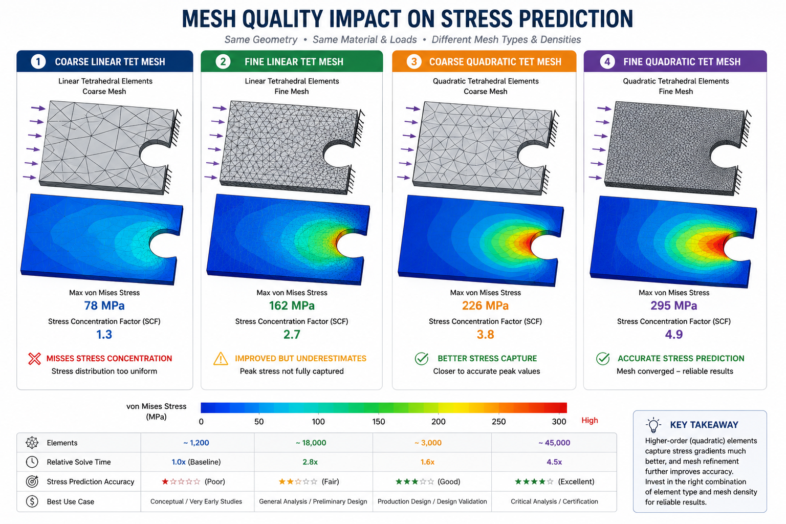
An engineer running FEA on a bracket that will carry a cyclic load has a stress concentration at a fillet radius. The linear analysis runs in three minutes and the peak stress reads 180 MPa. The material yield strength is 250 MPa. The result looks reasonable. The bracket goes into service and fails at the fillet in fatigue after six months.
A post-mortem examination finds a stress concentration factor of 3.2 at the fillet. The true peak stress was approximately 576 MPa, well above yield, producing plastic strain accumulation and fatigue damage with every cycle. The FEA result of 180 MPa was not a modeling error in the traditional sense. The boundary conditions were correct, the material was correctly specified, the load was accurately applied. The error was in the mesh: coarse linear tetrahedral elements at the fillet, unable to capture the steep stress gradient, averaging out the peak and reporting a smooth, conservative-looking 180 MPa where the true peak was more than three times higher.
This scenario, or close variants of it, represents one of the most common categories of consequential FEA error in practice. It is preventable with mesh quality knowledge, and that knowledge is what this article provides. It covers what mesh quality metrics mean at a mathematical level, what numerical phenomena cause mesh quality to degrade results, how to select element types correctly, how to perform mesh convergence studies that verify your results are mesh-independent, and how to handle the specific problem of stress singularities that confuse the convergence picture for sharp geometric features.
Why Mesh Quality Matters: The Mathematical Foundation
Finite element analysis works by dividing a continuous structure into discrete elements, approximating the displacement field within each element using shape functions (also called interpolation functions or basis functions), and assembling the element equations into a global system of equations that is solved for the nodal displacements. Stresses and strains are then computed from these displacement solutions using the element’s strain-displacement and stress-strain relationships.
The accuracy of this approximation depends fundamentally on how well the element’s shape functions can represent the true displacement field within that element. Shape functions are polynomial functions defined in a natural (idealized) coordinate system for a perfect element shape. When the element’s physical shape deviates from the ideal, the mapping between the natural coordinate system and the physical coordinate system introduces additional terms in the strain-displacement relationship that the ideal shape function formulation did not account for. These additional terms are the source of mesh-quality-induced error.
The Jacobian Matrix: Where Shape Quality Becomes Mathematical
The Jacobian matrix is the key mathematical link between an element’s physical shape and the accuracy of its numerical integration. It is the matrix of partial derivatives of the physical coordinates (x, y, z) with respect to the natural coordinates (xi, eta, zeta) of the idealized element. For a perfectly shaped element (square quad, equilateral triangle, regular tetrahedron, cube), the Jacobian matrix is constant throughout the element and its determinant, the Jacobian determinant, is constant and positive.
When an element is distorted (stretched, skewed, or warped), the Jacobian matrix varies across the element. If the distortion is severe enough, the Jacobian determinant can approach zero or even become negative at integration points within the element. A negative Jacobian indicates an inverted element: the element’s physical shape has been distorted so severely that the natural-to-physical mapping is no longer one-to-one. An inverted element will cause the FEA solver to either crash outright or produce completely incorrect results at that element’s location.
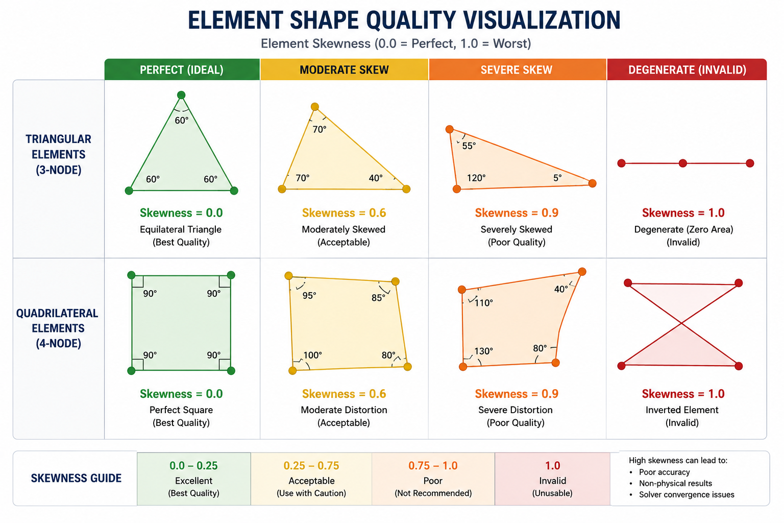
Between the ideal (Jacobian = 1.0 everywhere) and the inverted (Jacobian < 0.0) cases lies a spectrum of degraded accuracy. Jacobian values below 0.6 at any integration point indicate that the element shape distortion is significant enough that the shape function approximation is meaningfully compromised. Most professional FEA solvers (Ansys, Abaqus, Nastran, MSC Marc) flag elements below this threshold as potentially problematic and will warn the analyst. Some solvers allow the analyst to set the minimum acceptable Jacobian below which the analysis will be aborted.
Strain-Displacement Error: Why Aspect Ratio Matters
The aspect ratio of an element (the ratio of its longest edge to its shortest edge) directly affects the accuracy of the strain-displacement relationship within the element. In a well-shaped element with an aspect ratio near 1.0, the shape functions accurately interpolate both displacements and their spatial derivatives (strains) throughout the element volume. In a high-aspect-ratio element (an elongated or stretched element), the shape functions accurately capture displacement variation along the long axis but poorly capture variation along the short axis.
For structural FEA, this directional error in strain capture becomes critical in bending-dominated behavior. A beam element in bending has steep strain gradients across its thickness (the short dimension) and shallow gradients along its length (the long dimension). An elongated element aligned along the beam’s length will poorly capture the through-thickness strain gradient, underestimating the bending stiffness and the peak bending stress. This is why element aspect ratios above 5:1 in bending-dominated regions are considered problematic, while ratios up to 20:1 or even higher may be acceptable in membrane-dominated regions where the strain variation is aligned with the long element axis.
Mesh Quality Metrics: Thresholds, Meanings, and Measurement
Every major FEA solver provides mesh quality checking tools that compute and display quality metrics for every element in the model. Understanding what each metric measures, what the acceptable ranges are, and how violations of each metric affect the results is essential for interpreting these quality reports and deciding which elements need to be improved.
Metric
What It Measures
Ideal Value
Warning Threshold
Failure Threshold
Effect of Violation
Aspect Ratio
Ratio of longest to shortest element edge
1.0 (equilateral)
5:1 (hex/tet general)
10:1+ or 20:1 (bending-dominated)
Stiffness overestimation in bending; numerical ill-conditioning at high ratios
Jacobian (Normalized)
How well element shape maps from natural to physical coordinates
1.0 (perfect shape)
0.6 minimum (most solvers)
<0.0 (inverted element – always fix)
<0.6: shape function errors; <0.0: solver crash or completely wrong results
Skewness
Angular deviation of element from ideal shape
0.0 (no skew)
0.85 for FLUENT; 0.90 for structural
0.95+ (always fix)
Interpolation error in stress/strain; poor convergence in high-gradient regions
Severe interpolation errors; locking or excessive flexibility
Element Size Ratio (growth rate)
Transition rate between fine and coarse mesh regions
1.0-1.2 between adjacent elements
2.0 max in stress gradient regions
5.0+ (abrupt transition)
Stress discontinuity at mesh transitions; missed peak stress
Orthogonal Quality (Fluent CFD)
Element face orientation relative to flow direction
1.0 (best)
0.1 minimum
<0.01 (critical)
Diffusion errors in CFD; incorrect boundary layer resolution
How to Use This Table in Practice
The thresholds in this table are general guidelines, not absolute rules. The appropriate threshold depends on the analysis type, the solver being used, and the location of the element in the model. An element in a low-gradient region (far from stress concentrations, in a region dominated by uniform loading) can tolerate worse quality metrics than an element at a stress concentration or in a region with steep gradients.
The most important rule: zero inverted elements (negative Jacobian) in any final analysis mesh. This is the one mesh quality violation that is unambiguous: an inverted element always produces incorrect results and should always be corrected before running the analysis. All other quality metrics involve a judgment call based on the acceptable error level for the specific application, but negative Jacobian elements have no acceptable level.
Element Type Selection: The Decision That Precedes Mesh Quality
Before mesh quality metrics become relevant, the engineer must choose the element type for the analysis. This decision, made before the first element is created, determines the theoretical accuracy ceiling that even a perfect mesh can achieve. A mesh of perfectly shaped elements of the wrong type will produce results that are less accurate than a good mesh of the right type, regardless of how well the quality metrics score.
Element Type
DOF per Node
Captures Bending?
Accuracy vs Cost
Best Use Case
Avoid For
Linear Tet (C3D4/TET4)
3
No (constant stress)
Very poor accuracy for its cost
Never use alone for stress analysis
Any stress analysis – always use quadratic tet instead
Thick cross-sections, high shear-to-bending ratio applications
The Linear Tetrahedral Element: Why You Should Almost Never Use It
The linear tetrahedral element (C3D4 in Abaqus, TET4 in general) is the most commonly misused element in FEA practice. It is easy to generate automatically from CAD geometry using any commercial meshing tool, it creates meshes quickly, and it produces a solver file that runs without errors. For all of these reasons, it is the default element in many automatic meshing workflows, and for all of these reasons, it is a poor choice for structural stress analysis.
The linear tet element has only four nodes, each at a corner of the tetrahedron, and a constant stress field throughout the element volume. The displacement varies linearly from node to node, and because stress is the derivative of displacement, a linearly varying displacement produces a constant (zero-order) stress within each element. This means that a stress gradient across a region requires many elements to approximate, and the predicted peak stress is always an average over the element rather than a true point value. At a stress concentration, a linear tet mesh systematically underestimates the peak stress because the constant stress element cannot capture the steep gradient.
The quadratic tetrahedral element (C3D10 in Abaqus, TET10 in general) adds six mid-side nodes to the four corners, giving ten nodes total and a quadratic displacement field within the element. Because the displacement is quadratic, the stress (its derivative) is linear, meaning the stress can vary from corner to corner within a single element. This fundamentally different capability means that a quadratic tet mesh with the same element density captures stress gradients and stress concentrations dramatically better than a linear tet mesh. For complex organic geometry where hex meshing is impractical, the quadratic tet is the correct choice.
The Hourglassing Problem in Reduced-Integration Elements
Reduced-integration hexahedral elements (C3D8R in Abaqus, SOLID185 in Ansys) use one integration point at the element center rather than the full 2x2x2 = 8 integration point scheme of full-integration elements. This halves the computational cost of the element stiffness calculation, making them efficient for large models. However, reduced integration introduces a specific failure mode called hourglassing or zero-energy modes: deformation modes of the element that produce no strain energy at the single central integration point and therefore produce no restoring stiffness.
Hourglassing appears in the solution as a characteristic zig-zag displacement pattern visible in the deformed mesh, where alternating elements displace in opposite directions with very large magnitudes. The solution diverges from physical reality while the solver reports convergence (because the energy residual is still small, just distributed in a physically meaningless deformation pattern). Modern solvers include hourglass control algorithms that add artificial stiffness to resist the zero-energy modes, but these algorithms involve a user-defined scale factor that can either under-control (allowing hourglassing to corrupt results) or over-control (adding artificial stiffness that affects the real structural response).
The safest approach: use reduced-integration elements only when hourglass control is well-calibrated for the specific analysis type (dynamic explicit analyses where hourglassing is well understood and controlled, forming simulations where the software vendor has verified the hourglass control parameters), or switch to full-integration elements where hourglassing is not possible. For static stress analysis of structures where the mesh is not excessively distorted, full-integration elements are generally preferred despite their higher computational cost.
Mesh Convergence Studies: The Only Way to Know Your Results Are Reliable
The most important mesh quality verification tool available to every FEA analyst is the mesh convergence study: a systematic process of refining the mesh and comparing results across refinement levels to determine whether the results have converged to a mesh-independent value. A result that changes significantly as the mesh is refined is not reliable, because the level of refinement determines the answer rather than the physics. A result that stabilizes as the mesh is refined demonstrates that the mesh is fine enough to capture the relevant physics and that further refinement would not change the result meaningfully.
The Convergence Study Protocol
Identify the quantity of interest (QoI): Before meshing, identify the specific result that must be accurate: peak von Mises stress, maximum deflection, natural frequency, reaction force, temperature at a specific location. Mesh convergence is always with respect to a specific QoI, because different quantities converge at different rates with mesh refinement.
Create an initial coarse mesh: Generate the first mesh at a deliberately coarse element size. This is not the mesh you will use for the final analysis; it is the starting point for the convergence study.
Extract and record the QoI: Run the analysis on the coarse mesh and record the QoI value, the element count, and the total solve time.
Refine globally or locally: Reduce the element size by a factor of 2 (halving the mesh size in each dimension multiplies the element count by roughly 8 for 3D solid meshes). This is the h-refinement approach. Alternatively, increase the element polynomial order (p-refinement) while keeping the mesh coarse.
Repeat and plot convergence: Run the refined mesh, record the QoI, and plot QoI versus element count (or element size). Continue refining until the change in QoI between successive refinements is below a specified convergence criterion.
Apply Richardson extrapolation: Using two or more refinement levels, apply Richardson extrapolation to estimate the exact solution value and the discretization error. This provides a quantitative uncertainty estimate for the result rather than a qualitative judgment about whether the curve looks flat.
Mesh Convergence Convergence Criterion and Richardson Extrapolation CONVERGENCE CRITERION: Change in QoI from mesh N to mesh N+1 < 5% (engineering acceptable) Change in QoI from mesh N to mesh N+1 < 2% (high confidence) Change in QoI from mesh N to mesh N+1 < 1% (precision required)
RICHARDSON EXTRAPOLATION (2-level): Given: QoI_1 at mesh size h1, QoI_2 at mesh size h2 = h1/2 Estimated exact value: QoI_exact = QoI_2 + (QoI_2 - QoI_1) / (2^p - 1) where p = convergence order (p=2 for linear elements, p=3+ for quadratic)
Recommendation: Level 4 is adequate for engineering decisions. Level 5 adds 8x more elements for 0.9% additional accuracy.
h-Refinement vs p-Refinement vs hp-Refinement
Three mathematically distinct strategies exist for improving mesh accuracy: h-refinement reduces the element size (more, smaller elements of the same type), p-refinement increases the polynomial order of the element shape functions (same mesh, higher-order elements), and hp-refinement applies both simultaneously in a coordinated manner.
For smooth problems without singularities, p-refinement converges much faster than h-refinement: doubling the polynomial order of the elements reduces the error by a factor of 2^p, whereas halving the element size reduces the error by a factor of 2^p (where p is the order of the current elements). For a linear element mesh (p=1), halving the element size reduces the error by a factor of 4. For a quadratic element mesh (p=2), raising to cubic (p=3) may reduce the error by a factor of 8 for the same computational investment.
For problems with stress singularities (sharp corners, crack tips, contact edges), neither h-refinement nor p-refinement converges the local stress to a finite value, because the true solution has an unbounded stress gradient at the singularity. These cases require either singularity enrichment elements (special elements with the correct singular displacement field built into the shape functions, used in fracture mechanics), or deliberate exclusion of the singularity point from the convergence study, reporting the stress at a location removed from the singularity rather than at the singular point itself.
Stress Singularities: Where Mesh Convergence Studies Mislead
One of the most important and most frequently misunderstood aspects of FEA mesh quality is the stress singularity: a location in the model where the mathematical solution for the stress field approaches infinity, even though the real physical stress is finite. Stress singularities occur at sharp internal corners (re-entrant corners), at point loads or point constraints, and at crack tips in fracture mechanics problems. Every engineer using FEA must understand why singularities occur and how to handle them correctly.
Why Sharp Corners Produce Infinite Stress in FEA
Classical elasticity theory, which FEA implements numerically, predicts unbounded stress at sharp geometric re-entrant corners. This prediction is mathematically correct within the theory, but it does not represent a physical impossibility: in reality, every sharp corner has a finite radius (even if very small), every real material has a finite yield strength that prevents unbounded stress accumulation, and in fatigue design the relevant quantity is not the point stress at the corner but the stress in the process zone around it.
In an FEA model with a sharp internal corner, as the mesh is refined toward the corner, the peak stress continues to increase without bound. A convergence study at the corner node will show stresses that grow with every mesh refinement level and never converge to a stable value. An engineer who does not recognize this pattern may interpret the lack of convergence as a signal that the mesh needs further refinement, when in fact the correct response is to change the modeling strategy: add a fillet radius to the model geometry, or extract the stress at a location removed from the singularity using a Saint-Venant distance criterion.
The Saint-Venant Principle for Practical Stress Extraction
Saint-Venant’s principle states that the stress distribution at a cross-section far enough from a localized load or constraint is essentially independent of the exact distribution of that load. In FEA practice, this principle is applied to singularities: the stress at a distance from the singular point equal to the largest characteristic dimension of the stress perturbation is mesh-independent and physically meaningful, even though the stress at the singular point itself is not.
For a re-entrant corner in a plate under tension, the stress approximately one fillet-radius distance away from the corner is mesh-converged and corresponds to the local stress that governs fatigue initiation in the real structure. This is the quantity to extract and report, not the stress at the corner node itself. Most FEA guidelines for fatigue assessment of welded structures, pressure vessels, and aerospace structures define hot spot stress or structural stress methodologies that explicitly extract stress at defined distances from the geometric discontinuity for exactly this reason.
Adaptive Meshing: Automating the Convergence Process
Adaptive mesh refinement (AMR) is an FEA capability that automates the convergence study by computing an error estimate at each element, identifying elements where the error estimate exceeds a target threshold, and automatically refining those elements before solving again. The process iterates until all elements meet the error target. The result is a mesh that is fine where the physics demand it and coarse where coarse elements are adequate, without the engineer having to manually identify and refine high-error regions.
Error Estimators: How the Software Knows Where to Refine
Adaptive meshing requires an error estimator: a mathematical measure of how much error is present in each element’s solution. The most common type is the stress discontinuity error estimator, based on the observation that in an exact FEA solution, the stresses should be continuous across element boundaries. In a mesh of finite elements, the stresses are computed independently in each element and are generally discontinuous at the element boundaries. The magnitude of this stress discontinuity at each element boundary is proportional to the error in the adjacent elements.
The Zienkiewicz-Zhu (ZZ) error estimator is the most widely implemented in commercial FEA software. It computes a smoothed, continuous stress field by averaging the element stress values at each node, then computes the difference between the smoothed field and the element-level field at each integration point. The norm of this difference is the element error indicator. Elements with high error indicators are refined in the next adaptive cycle. The ZZ estimator is available in Ansys (as the Energy Norm Error tool), in Abaqus (as the error indicators for mesh-to-mesh solution mapping), and in Nastran (as the mesh sensitivity study tools).
When Adaptive Meshing is and Is Not Appropriate
Adaptive meshing is most effective for smooth problems without singularities: structural analysis of continuous components with smooth geometry under smoothly varying loads. In these cases, the error estimator correctly identifies regions of high error, the mesh refinement reduces that error efficiently, and the process converges to a well-distributed mesh with predictable accuracy.
Adaptive meshing is less effective for problems with singularities because the error estimator correctly identifies the singularity as a high-error region and will attempt to refine it indefinitely. Most adaptive meshing implementations include maximum refinement limits to prevent infinite refinement at singularities, but the result is typically a very fine mesh concentrated at the singularity that does not improve the physically meaningful stress result because the true solution at the singularity is unbounded. For these problems, the engineer must either remove the singularity by geometric modification (adding a fillet) or apply the Saint-Venant extraction strategy manually.
Platform-Specific Mesh Quality Guidance
Each major FEA platform has its own implementation of mesh quality checking, quality metric naming conventions, and default threshold settings. Knowing the specific tools in your platform and how to interpret their outputs prevents the confusion that arises when metric names or thresholds differ between platforms.
Ansys Mechanical
Ansys Mechanical provides mesh quality metrics under Mesh > Mesh Quality. The primary metrics available include: Element Quality (a composite metric from 0 to 1, target > 0.5 for most elements), Aspect Ratio (target < 5 for most analyses), Jacobian Ratio (target > 0.6 at all integration points, > 0 required), Warping Factor (target < 0.4 for shell elements), Maximum Corner Angle (target < 170 degrees), and Skewness (target < 0.9 for structural, < 0.85 for thermal/CFD).
The Ansys mesh quality report displays histograms of each metric and allows the engineer to visually identify elements below threshold. The Named Selections feature allows poor-quality elements to be selected, inspected, and manually remeshed using local mesh controls (sphere of influence, edge sizing, face sizing) without remeshing the entire model.
Abaqus/CAE
Abaqus uses the Verify Mesh tool (Mesh menu > Verify) to check element quality. Abaqus reports: warnings for elements where the Jacobian at any integration point is between 0 and the user-defined warning threshold (default 0.1), errors for elements with negative Jacobian, and analysis checks for elements where the aspect ratio exceeds the warning threshold. Abaqus additionally provides error indicators as output variables (ENDENERI, ESEDEN) that can be plotted as contour maps to visualize where mesh refinement would most improve the solution accuracy.
Siemens NX Nastran
Nastran provides the DMIG (Direct Matrix Input at Grid points) and PBARL/PBEAML beam cross-section quality metrics, but mesh quality checking for solid and shell elements is primarily performed in the pre-processor (Femap, NX Meshing) before the Nastran analysis is run. The pre-processor provides element quality checks including Jacobian, aspect ratio, warpage, taper, and interior angle checks with thresholds that can be customized for the specific Nastran solver version and analysis type. Nastran CBUSH and RBE element quality is checked separately through model validation routines that verify constraint consistency.
Frequently Asked Questions
Q: What is mesh quality in FEA and why does it matter?
Mesh quality in FEA describes how well the shape, size, and distribution of the finite elements approximate the geometry and physics of the problem being analyzed. Poor mesh quality degrades accuracy because finite element shape functions are derived for ideally shaped elements. When elements are distorted (high aspect ratio, skewed, or warped), the shape function approximation introduces errors in the computed strain and stress fields. The most critical quality metric is the Jacobian: an element with a negative Jacobian (inverted element) is always incorrect and must be fixed. Elements with Jacobian below 0.6 may produce inaccurate results in high-gradient regions.
Q: What is an acceptable aspect ratio for FEA mesh elements?
For general structural analysis, aspect ratios below 5:1 are acceptable for most element types. In bending-dominated regions, ratios above 5:1 can cause underestimation of bending stiffness and peak stress because the short-axis strain gradient is poorly captured. In membrane-dominated regions where the strain variation aligns with the long element axis, ratios up to 20:1 may be acceptable. For shell elements in the bending direction (through-thickness), at least 4 elements are typically required to capture the stress gradient accurately, which implies aspect ratios should be kept below 5:1 in the critical direction even if the overall element aspect ratio is higher.
Q: Should I use tetrahedral or hexahedral elements for structural FEA?
Quadratic tetrahedral elements (10-node tet) are generally the better choice for complex organic geometry because they can be generated automatically from CAD geometry and provide good accuracy with a reasonable element count. Linear tetrahedral elements (4-node tet) should almost never be used for structural stress analysis because their constant stress field systematically underestimates stress concentrations. Hexahedral (brick) elements provide the best accuracy per degree of freedom but require structured or semi-structured meshing that is time-consuming for complex geometry. The practical recommendation: use quadratic tet for complex geometry, use hex where geometry allows structured meshing and maximum accuracy is required.
Q: What is a mesh convergence study and how do I perform one?
A mesh convergence study is a systematic process of refining the mesh and tracking the change in a specific result quantity (peak stress, maximum deflection, natural frequency) across refinement levels. When the result changes by less than a specified percentage (typically 5% for engineering decisions, 2% for high-confidence analysis) between successive refinements, the mesh is considered converged. The process involves creating 3 to 5 mesh refinement levels with progressively smaller elements, running the analysis at each level, plotting the result versus element count, and checking whether the curve has plateaued. Richardson extrapolation can be applied to estimate the exact value and quantify the remaining discretization error.
Q: What is a stress singularity in FEA and how do I handle it?
A stress singularity is a location in the FEA model where the mathematical stress solution is unbounded (approaches infinity), even though the real physical stress is finite. Singularities occur at sharp re-entrant corners, at point loads, at point constraints, and at crack tips. In an FEA model with a singularity, the predicted stress at the singular point increases without bound as the mesh is refined, and a convergence study at that location will never converge.
The correct handling depends on the context: add a physical fillet radius to represent the real geometry, extract the stress at a distance from the singularity using Saint-Venant’s principle, or use specialized fracture mechanics elements at crack tips. Never report the stress value at a singular point as a meaningful result.
Q: What is hourglassing in FEA and how do I prevent it?
Hourglassing (also called zero-energy modes or kinematic modes) is a numerical instability that occurs in reduced-integration elements (elements using fewer integration points than the full integration scheme). The reduced integration point scheme fails to detect certain deformation modes (the hourglass modes) because these modes produce no strain at the single central integration point. The solution exhibits a characteristic checkerboard pattern of displacements with large magnitudes that is entirely non-physical. Modern solvers include hourglass control that adds artificial stiffness to resist hourglass modes. To prevent hourglassing: use full-integration elements in static stress analysis, use at least two or three elements through any thin-walled section, and review the deformed mesh carefully for checkerboard patterns after any analysis using reduced-integration elements.
Conclusion:
Every quality metric, threshold, and guideline in this article is a tool for engineering judgment, not a substitute for it. The mesh quality checker that reports all elements above 0.6 Jacobian and below 5:1 aspect ratio has done its job, but it cannot tell you whether those elements are in the right places, whether the mesh is fine enough near the features that govern the structural response, or whether the convergence study has been correctly interpreted for a problem with stress singularities.
The engineering judgment is: identifying the critical regions before meshing (where are the stress concentrations, the load introduction points, the contact interfaces?), choosing element types appropriate for the dominant structural behavior, performing a convergence study with respect to the quantity that actually matters for the engineering decision, and correctly distinguishing converging results from singularity behavior. These judgments are what the quality metrics support and inform, but they are not substituted by the metrics.
An FEA result supported by a mesh convergence study that demonstrates less than 5 percent change between the final two refinement levels, with no inverted elements, no Jacobian values below 0.6 in high-gradient regions, and element type selection appropriate for the dominant structural behavior, is a result that can be defended in an engineering review and relied upon for a design decision. That is the standard the discipline demands and the standard this article has provided the tools to meet.
Every engineering team has the experience of watching a senior engineer produce a complex assembly in an afternoon while a junior engineer takes three days to produce something less complete. The difference is rarely intelligence or even technical CAD skill. It is almost always the compound advantage of reusable assets: templates that pre-populate the correct settings, library components that drop into place without being modeled from scratch, standard parts that carry all their properties, connections, and documentation already built in.
A well-built reusable CAD library is the infrastructure that makes engineering teams consistently faster, more consistent, and less error-prone than teams working without one. It is also one of the most consistently under-built assets in engineering organizations, not because teams do not understand its value, but because building it correctly requires deliberate architecture, governance discipline, and ongoing maintenance that feel like overhead in the middle of a delivery-focused project schedule.
The result of this underinvestment is a library built organically, one copied file and one downloaded model at a time, that grows into a collection of components with inconsistent quality, inconsistent naming, unknown reliability, and no governance. Engineers are never sure whether a library component is current, correct, or trustworthy. They start modeling from scratch, duplicating effort across the team, and the library’s potential value goes unrealized.
This article provides the architecture, the build process, the governance framework, and the platform-specific tool knowledge to build a CAD library that engineers actually use. It covers all six tiers of a complete library system, from drawing templates to supplier-provided geometry. It covers the validation workflow that keeps the library trustworthy. It covers the ROI calculation that justifies the investment to leadership. And it covers the lifecycle disciplines that keep the library healthy over years of active use.
Why Most CAD Libraries Fail Before They Deliver Value
The failure mode of a CAD library is almost always the same regardless of the organization, the CAD platform, or the industry. The library starts with good intentions and a burst of productive initial investment. A folder is created. Some templates are dropped in. A few downloaded models are added. An engineer contributes a part they just finished that might be useful to others. After six months, the folder has grown, but no one is entirely sure what is in it, how current any of it is, or whether the components were built to any standard.
The library becomes a secondary option rather than the default starting point. Engineers use it occasionally when they happen to know a relevant component exists, but they do not trust it enough to rely on it systematically. The productivity gains that motivated the initial investment are never realized.
The Trust Problem Is a Quality Problem
The root cause of library failure is almost always insufficient quality control at the point of entry. When any engineer can contribute any component to the library without review, the library inherits the quality level of the least careful contributor. When supplier-provided models are downloaded and placed in the library without validation, the library inherits whatever errors exist in those models. When templates are created once and never updated as standards evolve, the library drifts out of alignment with current practice.
Engineers are rational actors. When a library component has failed them once by producing a rebuild error, a wrong dimension, or an incorrect material property, they stop trusting the library. Once trust is lost, it is difficult to rebuild, because the history of past failures makes engineers skeptical of even the correctly built components that exist alongside the problematic ones.
The Library Contamination Problem
Library contamination is what happens when a poorly built component enters the library and is reused across multiple projects before the error is discovered. A fastener with an incorrect thread pitch. A bearing with the wrong bore tolerance. A standard bracket with a dimension that was correct for the project where it was originally designed but is wrong as a general standard. Each use of the contaminated component spreads the error further, and when the problem is eventually discovered, the correction must be applied across every project that used the component.
The contamination problem is geometrically more damaging than a single modeling error because it multiplies. An error that affects one part in one project costs one engineer some hours to fix. The same error in a library component used in twenty projects across two years costs twenty times as much to find and correct, plus the investigation time to identify every instance of use. This is why the quality gate at library entry is not bureaucratic overhead. It is a compounding investment in error prevention.
The Fundamental Principle A CAD library is only as valuable as the trust that engineers place in it. Trust is earned by quality control at entry and maintained by governance over time. A library that is fast to build but low in quality will be used sparingly and will deliver a fraction of its potential value. A library that is slower to build but rigorously controlled will be used as the default starting point and will deliver compounding productivity returns across every project that uses it.
The Six-Tier Library Architecture: A Framework That Scales
The most effective CAD libraries are not flat collections of files. They are structured in tiers that correspond to different types of reusable assets, each with its own creation process, its own governance rules, and its own use pattern. Understanding this tier structure is the prerequisite for building a library that remains organized, trustworthy, and useful as it grows.
Library Tier
Content Type
Who Creates
Who Uses
PDM Control Level
Tier 1: Templates
Part, assembly, drawing templates with pre-set standards
Mixing asset types in a flat library structure creates confusion about what each file is for and how it should be used. A drawing template and a fastener model look identical in a folder view, but they serve completely different purposes, require different creation processes, and carry different governance requirements. Separating them into explicit tiers makes the library navigable, makes governance rules clear, and makes the contribution process unambiguous for engineers who want to add new assets.
Tier separation also allows different governance strictness at each level. Tier 1 templates and Tier 3 standard hardware must be locked and admin-controlled because an error in these assets propagates to every new file and every assembly in the organization. Tier 4 custom standard components can have lighter governance because they are less universally applied. Tier 6 reference geometry can be project-specific and does not need to meet library quality standards because it serves a narrow, well-understood purpose within one project context.
Tier 1: Building the Template Layer That Everything Else Depends On
Templates are the foundational layer of the library and the highest-leverage asset in it. Every part file, every assembly, every drawing that any engineer creates in your organization starts from a template. A well-designed template pre-configures every standard setting that would otherwise require manual setup: the unit system, the document properties, the custom property fields, the material database connection, the drawing sheet format, the title block, and the default view scale. An engineer opening a correct template is seconds away from productive work. An engineer setting up a new file from scratch is ten to thirty minutes away.
What a Complete Part Template Contains
A production-ready part template is not just a blank part file saved as a template. It is a pre-configured engineering document that enforces your team’s standards automatically. Before the engineer draws a single line, the template has already done the following:
Unit system: Millimeters and kilograms, or inches and pounds, set at the document level and impossible to accidentally change without explicitly overriding the template setting.
Custom property fields: Part number, description, material, surface finish, revision, drawn-by, approved-by, and any other properties that feed the drawing title block or the BOM. Every field exists and is labeled correctly from the moment the file is created.
Material database linked: The material library is connected so engineers can select materials from the approved list rather than typing free-form text that creates BOM inconsistencies.
Reference geometry pre-built: The three standard reference planes are named according to your team convention (Top, Front, Right or XY, YZ, XZ depending on your standard) rather than the CAD tool’s default names that vary between platforms.
Feature tree started: An origin folder, any company-standard reference geometry that belongs in every part, and any annotation notes that must appear in every model are already present.
Default display settings: Edge display, face color convention, and any visual standards that the team applies uniformly are pre-set so every model looks consistent without engineer intervention.
What a Complete Drawing Template Contains
The drawing template is the most visible template in the library because it is what suppliers, manufacturing, quality, and customers see. Its configuration directly affects the professional presentation of every engineering document the team produces.
Title block: Fully formatted with all mandatory fields, linked to the model’s custom properties so that part number, description, revision, and other fields auto-populate when the drawing is created.
Sheet formats: Multiple sheet sizes (A4, A3, A2, A1, or B, C, D, E depending on your region) pre-formatted with your logo, border, and title block at the correct scale.
Dimensioning standards: ASME Y14.5 or ISO 1101 annotation standards set at the document level so that all GD&T symbols, datum triangles, and feature control frames use the correct symbol set automatically.
Layer or display state standards: Pre-configured layers for dimensions, notes, centerlines, and hidden lines with the correct line weights and styles for your organization’s drawing standard.
Note blocks: Any standard notes that appear on every drawing, such as general tolerance callouts, surface finish standards, or material specification formats, are already placed and formatted.
Setup Investment vs. Return A complete set of part, assembly, and drawing templates for a mechanical engineering team takes two to three days to build correctly. Once built and deployed through the PDM system, those templates save every engineer in the team 20 to 30 minutes on every new file they create. For a team of ten engineers creating five new files per week each, the template investment breaks even in approximately two weeks and continues delivering returns indefinitely.
Tier 2: Library Features, UDFs, and iFeatures for Reusable Geometry Patterns
Between templates (which set up a file) and full part models (which are complete components) sits a middle tier of reusable assets that most engineers are unaware of: library features. A library feature is a reusable geometry pattern that can be inserted into any part at any location, sized according to the local geometry, and positioned as needed. It is not a complete part. It is a parametric geometry recipe that can be applied to many different parts.
The most obvious example is a fastener hole pattern. Every time an engineer creates a counterbored hole for an M8 socket cap screw, they perform the same sequence of operations: a circular sketch, an extrude-cut for the clearance diameter, another extrude-cut for the counterbore diameter, and a depth specification for each. A library feature encapsulates this entire sequence into a single drag-and-drop operation. The engineer drags the M8 clearance hole library feature onto a face, specifies the depth, and the full hole geometry is created in one step.
SolidWorks Library Features
SolidWorks Library Features are saved as .sldlfp files and stored in a location configured as the library feature folder in the SolidWorks options. They appear in the Design Library task pane and can be dragged directly onto faces in the active part. A library feature can include multiple features (the sketch plus the two cuts in the counterbore example), references (the face to apply the feature to), and configurable dimensions (the hole depth, the edge distance) that the engineer specifies during placement.
Effective SolidWorks Library Features are built with reference geometry that allows flexible placement: a reference point that can be positioned anywhere on the target face, dimensions that reference the feature’s own geometry rather than the parent part’s geometry so they remain valid regardless of where the feature is placed. Library features that are rigidly anchored to specific coordinates in their host part will not transfer correctly to different parts with different geometries.
PTC Creo User-Defined Features (UDFs)
Creo UDFs (User-Defined Features) function similarly to SolidWorks Library Features but with stronger parameterization capabilities. A UDF is saved as a standalone feature file and can be referenced by any Creo part file. When placed, the UDF prompts the engineer to specify the reference geometry (the face, edge, or datum to anchor the feature to) and any variable dimensions. Creo UDFs support dependency references, meaning the placed feature can reference existing geometry in the host part for size calculations, enabling more adaptive placement behavior than is typically achievable with SolidWorks Library Features.
Creo also supports Group UDFs, which combine multiple features into a single reusable group that can be propagated to all members of a Family Table simultaneously, making UDFs a natural companion to the configuration management workflows common in Creo-based engineering environments.
Autodesk Inventor iFeatures
Inventor iFeatures are the Inventor equivalent, stored as .ide files in the iFeatures folder configured in Inventor’s project settings. Like UDFs and Library Features, iFeatures capture parametric geometry patterns and allow flexible placement. Inventor’s iFeature creation process is particularly well-integrated with the Inventor design environment, allowing features to be extracted from existing parts by selecting them in the feature tree and using the Create iFeature command rather than building the feature from scratch in a separate file.
This extraction approach is valuable for teams migrating to a library-first workflow: instead of starting from scratch, engineers can extract the best-built examples of common feature patterns from recent designs and convert them directly into iFeatures for the library. This both populates the library quickly with high-quality examples and establishes the quality standard that future library contributions should meet.
Tier 3: Building the Standard Hardware Library Correctly
Standard hardware, fasteners, bearings, seals, springs, and connectors, is the component category that teams most commonly try to address through external download sources. Sites like 3D ContentCentral, TraceParts, and McMaster-Carr provide downloadable models for millions of standard parts. The temptation is to download whatever is needed at the moment and add it to the library. This approach is faster to start but creates the quality and consistency problems that make the library untrustworthy over time.
The Supplier Model Validation Workflow
Every model that enters the standard hardware library from an external source must pass through a validation workflow before it is available for use. This workflow is not optional. Its purpose is to prevent library contamination from supplier models that have incorrect dimensions, missing mass properties, incorrect material assignments, or geometry errors that cause assembly interference problems.
The validation workflow for each supplier model should include the following steps, performed by a designated validator before the model is committed to the library:
Dimensional verification: Open the model and check its key dimensions against the supplier’s published specification sheet or datasheet. Verify the thread pitch, the bore diameter, the overall envelope, and any critical interface dimensions. A bearing whose bore diameter is wrong by 0.1 mm will cause every assembly that uses it to have an interference error.
Mass properties check: Verify that the model’s reported mass is consistent with the supplier’s published weight specification. A model with zero mass or obviously incorrect mass has not been assigned material properties, and any assembly that includes it will have incorrect mass calculations.
Geometry integrity check: Run the CAD platform’s geometry check tool (Check Entity in SolidWorks, Geometry Check in Creo) to verify that the model contains no invalid geometry, non-manifold edges, or zero-thickness faces that would cause assembly or analysis errors.
Property population: Add all standard custom properties: part number, supplier name, description, material, mass, and any other properties that your team’s BOM requires. A model with empty property fields will produce BOM line items with missing data.
Reference geometry alignment: Verify that the model’s origin and reference planes are positioned in a way that makes assembly mating intuitive. A bolt whose origin is at the tip of the thread rather than at the head face will be awkward to mate correctly in assemblies.
Simplification review: Assess whether the model’s geometric complexity is appropriate for its intended use in assemblies. Supplier models sometimes include internal geometry, thread detail, and surface features that are accurate but create enormous file sizes and slow assembly performance. Simplify or defeature before adding to the library if the model will be used in large assemblies.
Building Parametric Fastener Tables in the Library
Rather than downloading and validating individual fastener models for every size that might be needed, a more scalable approach is to build parametric fastener part files with design tables that cover an entire size range from a single model. A single parametric M-series socket cap screw model driven by a design table can produce M3, M4, M5, M6, M8, M10, M12, M16, and M20 configurations from one file, each configuration with the correct dimensions, mass, and properties for that size.
This approach reduces the library file count, ensures dimensional consistency across the size family (since all sizes are derived from the same parametric model), and makes adding a new size trivial (add a row to the design table). The initial investment to build the parametric model and populate the design table for a complete M-series range is two to three hours, after which the entire size family is available indefinitely with no further modeling work.
Tier 4: Custom Standard Components and Sub-Assemblies
Custom standard components are the most company-specific layer of the library and often the most valuable. They are the parts and sub-assemblies that appear repeatedly across your company’s products because they represent solutions to problems that your engineering team has already solved well: a mounting bracket in three sizes, a standard cable clamp, a universal gearbox interface plate, a sensor mounting block that accommodates your standard sensor family. Every time an engineer needs one of these components, they should not be modeling it. They should be dragging it from the library.
Identifying Candidates for the Custom Library
The fastest way to identify candidates for the custom standard component library is to conduct a frequency audit: review the last twelve months of completed designs and identify parts or sub-assemblies that appear in more than one project. Any component that was modeled more than once represents a duplication of effort that a library component would have prevented. High-frequency repeats are the highest-priority library candidates.
A complementary approach is to look at the future product roadmap: which components are likely to be needed across multiple upcoming projects? Building these as library components before the first project that needs them means every subsequent project benefits from the library version rather than the project-specific version.
Building Custom Components for Reuse, Not Just for Use
A component designed for a specific project and a component designed for the library look different from the inside, even if their external geometry is identical. A library component is built with reuse explicitly in mind: named parameters for every dimension that might need to vary between applications, a design table to manage multiple standard configurations, descriptive feature naming that makes the model understandable to any engineer who opens it, fully populated custom properties that feed correctly into any project’s BOM, and a library-standard reference plane convention that makes mating in any assembly intuitive.
Building components for the library takes longer than building them for a single project because of this additional investment in parametric structure, documentation, and configuration. The additional investment is typically 50 to 100 percent more time than a project-specific part would require. This additional time is recovered the first time the component is reused from the library rather than rebuilt from scratch.
The Review and Approval Process for Custom Components
Custom components entering the library must pass through a review process that verifies their quality before they are available to the team. The review should be performed by a designated reviewer (the CAD manager, a lead engineer, or a rotating review role depending on team size) and should check:
Is the part built to the library modeling standard? Named parameters, logical feature tree, correct template used as the starting point?
Are all custom properties populated correctly and consistently with the library’s naming conventions?
Does the design table (if applicable) include all expected configurations and have all configurations been verified to rebuild correctly?
Is the reference geometry (origin planes, mating faces) positioned according to the library standard so the part mates correctly in any assembly?
Is the model simplified appropriately for assembly use? No unnecessary internal geometry, no thread detail that creates performance problems in large assemblies?
Is the component documented in the library register with its intended use, size range, applicable standards, and the contact for questions?
Library Governance: The System That Keeps the Library Trustworthy
A library without governance is a library with a deadline. It will be useful for a period, degrade gradually as inconsistent contributions accumulate and outdated components go uncorrected, and eventually become too unreliable for systematic use. Governance is what converts a one-time investment in library building into a long-term compounding asset.
The CAD Library Register
Every library component should have a corresponding entry in a library register: a controlled document that records what each library asset is, who is responsible for it, when it was last reviewed, and whether it is current and approved for use. The register does not need to be elaborate. A structured spreadsheet or a simple PLM record for each library component is sufficient for most teams.
Library_ID : Unique identifier (e.g., LIB-MECH-0042) Component_Name : Descriptive name matching library file name Tier : 1=Template | 2=LibFeature | 3=StdHardware | 4=Custom | 5=Supplier Category : Fasteners | Bearings | Seals | Brackets | Subassemblies | etc. File_Path : Controlled path within PDM vault Current_Revision : Library revision letter (A, B, C...) Status : Active | Under Review | Deprecated | Archived Owner : Engineer responsible for maintaining this component Last_Review_Date : Date of most recent quality audit Next_Review_Due : Scheduled next audit (typically annual) Known_Limitations : Any constraints on use or known issues Usage_Count : Number of projects using this component (tracked by PDM) Applicable_Standards: ISO/ASME/company standard this component conforms to Notes : Anything unusual about this component that users should know
The Library Audit Cycle
Schedule a library audit at regular intervals, at minimum annually, and ideally semi-annually for active libraries with frequent contribution. The audit reviews every active library component against the following questions:
Is this component still being used? Check the PDM usage tracking. Components with zero uses in the past twelve months are candidates for archiving.
Has the underlying standard, specification, or supplier catalogue changed since this component was added? If yes, update the component or flag for update.
Has a better version of this component been built as part of a recent project? If yes, evaluate whether the project version should replace or supplement the library version.
Are there any known issues or limitations that have been discovered since this component was approved? Document them in the register.
Is the component’s documentation current? Custom properties, notes, and library register entry should reflect the component’s current state.
Components that fail the audit are not necessarily deleted. They are moved to a review queue, corrected by their owner, and re-approved before being restored to active status. Components that cannot be corrected (because the underlying design is superseded or the responsible owner has left the organization) are deprecated, marked clearly as not for use in new projects, and eventually archived.
Contribution Workflow: Making It Easy to Add, Hard to Contaminate
The governance paradox in library management is that the stricter the contribution process, the fewer contributions the library receives, but the more trustworthy each contribution is. The looser the contribution process, the more contributions the library receives, but the less trustworthy each one is. The solution is to make the correct contribution path easy and the incorrect path difficult: streamline the review process so it takes hours rather than days, and configure the PDM system so that engineers cannot add files to the library folders without triggering the review workflow.
In practice, this means providing engineers with a contribution template: a checklist of what a library-ready component must include, a naming convention guide, and a simple submission process (check the file into a specific PDM folder that triggers the review workflow). The reviewer is notified automatically, completes the review against the checklist, and either approves the component (moving it to the active library) or returns it to the contributor with specific feedback on what needs to change.
PDM Integration: Making the Library the Path of Least Resistance
The most technically complete CAD library in the world delivers zero value if engineers cannot easily find and use what is in it. Library accessibility is a design decision, not just a storage decision. How the library is connected to the CAD environment, how engineers discover what is available, and how quickly they can go from knowing they need a component to having it in their assembly determines the actual usage rate of the library and therefore the return on the investment that built it.
Configuring the PDM Vault as the Library Source
In a PDM-managed environment, the library should live in the vault as a set of controlled, read-only folders that every engineer has access to through the PDM client. Engineers should never need to navigate outside their CAD tool to find library components: the library folder appears in the CAD task pane or design library panel, and components can be dragged directly from it into the active assembly.
SolidWorks PDM Professional integrates directly with the SolidWorks Design Library panel, making library files in the vault accessible through the same interface used to access local library files. Creo Windchill provides a similar integration through the Windchill workspace. Autodesk Vault integrates with the Inventor Place Component dialog. Configuring these integrations correctly is the single highest-return configuration task in library deployment, because it removes all friction between knowing a library component exists and using it.
Search and Discoverability: Engineers Must Be Able to Find What Exists
An inaccessible library component is a wasted investment. Every component in the library must be findable through search, not just through navigation. This requires populating the library register and component metadata with the terms engineers actually use when searching: not just the formal standard name of the component but the common names, abbreviations, and synonyms that engineers type into the search box at two in the afternoon when they need a part fast.
PDM systems with full-text search across custom properties provide the most comprehensive discoverability. Supplement the search capability with a visual catalog: a simple PDF or web-based gallery of library components organized by category, with thumbnail images and key specifications visible without opening the CAD file. Engineers browsing for a solution to a design problem often do not know the exact name of what they need. A visual catalog enables discovery by recognition in a way that text search alone cannot.
The Library Landing Page Concept
For larger teams, consider building a library landing page: an internal intranet page or shared document that serves as the human-readable index of the entire library. It lists every active library tier, provides links to the relevant PDM folder for each tier, includes the library register for reference, shows any recent updates or additions, and lists the CAD manager’s contact for library questions and contributions.
This landing page converts the library from a set of folders in a vault into an explicit team resource with a visible home. Engineers who know where the library landing page is and visit it regularly will use the library more consistently than engineers who must remember which PDM folder path contains the asset they need.
Library Component Lifecycle: When to Update, Fork, or Retire
Every library component has a lifecycle that does not end at the moment it is approved and made active. Components evolve as designs improve, as standards update, as manufacturing processes change, and as the team’s understanding of a problem domain deepens. Managing this lifecycle correctly is what separates a library that improves over time from one that gradually accumulates obsolete versions.
When to Update a Library Component
Update a library component when a better version of the same solution exists: the original had a modeling error, the underlying standard has been revised, or a recent project produced a clearly superior implementation of the same function. Updates should always increment the revision letter, and the previous revision should be archived rather than deleted. Projects that used the previous revision should be tracked in the PDM system so that the engineering team can assess whether those projects need to update to the new library version.
Update decisions that affect widely-used components require communication to the team: a brief notice that library component LIB-MECH-0042 has been revised to revision B, with a summary of what changed and why, and guidance on whether existing projects using revision A need to update. Without this communication, engineers may continue using the revision A version without knowing a better version exists.
When to Fork a Library Component
Fork a library component when a project requires a variant that differs enough from the original to justify a separate library entry but shares enough commonality to warrant starting from the original as a base. A standard mounting bracket that needs a new size range, a standard seal groove that needs a different material specification for a high-temperature application, a standard connector block that needs a modified pinout for a new product platform.
Forking produces two library entries from one original. Both are active, both are governed, and both are documented in the register with a note indicating their relationship. The fork is not a copy of the original that then diverges uncontrolled: it is a deliberate, documented branching of the component’s lineage, with both branches maintained under the library’s governance process.
When to Retire a Library Component
Retire a library component when its underlying function has been superseded by a newer component that does the same job better, when the component is no longer used in new designs and is not expected to be needed in future projects, or when the component was built to a standard that is no longer applicable.
Retired components are not deleted. They are moved to an archived tier in the library with a status marking them as not for use in new projects, but available for reference in projects that used them historically. This archive respects the reality that engineers working on maintenance or warranty issues for older products may need to reference the exact component geometry that was used in the original design, even if that component is no longer appropriate for new work.
The ROI Calculation: Justifying the Library Investment to Leadership
Engineering managers asked to invest in building a CAD library need a return on investment analysis, not just a productivity narrative. The following table provides the framework for building that analysis using your team’s own numbers.
Activity
Without Library (hrs)
With Library (hrs)
Time Saved per Use
Break-Even at
Place a standard fastener in assembly
0.25 (model from scratch or find file)
0.02 (drag from library)
0.23 hrs (92% reduction)
4.5 uses
Add a standard bearing to assembly
1.5 (download, validate, place)
0.05 (validated, drag in)
1.45 hrs (97% reduction)
1 use
Start a new part with correct standards
0.5 (set up template properties manually)
0.02 (open template, rename)
0.48 hrs (96% reduction)
2 uses
Reuse a company-standard bracket
4 (model from scratch)
0.1 (drag, configure)
3.9 hrs (97% reduction)
1 use
Add a boss-and-counterbore feature
0.5 (sketch, extrude, cut sequence)
0.05 (drag Library Feature)
0.45 hrs (90% reduction)
2 uses
Start a new drawing with title block
0.5 (set up formats manually)
0.02 (open drawing template)
0.48 hrs (96% reduction)
2 uses
Library build investment (one component)
N/A
2-4 hrs (model, validate, document)
N/A
2-4 reuses to break even
To calculate your team’s specific ROI, take each activity row, estimate how frequently each engineer on your team performs that activity per month, multiply by the time saved per use, and sum across all engineers and all activities. For a team of eight engineers, the aggregate monthly time saving from a complete library implementation typically ranges from 40 to 120 engineering hours per month, depending on the nature of the work and the starting point of efficiency. At an engineering cost rate of 80 to 150 dollars per hour, this represents a monthly value of 3,200 to 18,000 dollars that the library delivers after breakeven.
The library build investment for a team of eight engineers starting from scratch is typically 80 to 160 hours across the CAD manager and contributing senior engineers, concentrated in the first three months and ongoing at 8 to 16 hours per month for maintenance and expansion. This investment breaks even within the first quarter for most teams and delivers compounding returns every month thereafter as the library grows and usage deepens.
Frequently Asked Questions
Q: What is a reusable CAD library and why does every engineering team need one?
A reusable CAD library is a curated, governed collection of templates, reusable geometry features, standard hardware models, custom standard components, and supplier-provided geometry that engineers can use directly in their designs without modeling from scratch. Every engineering team needs one because the same components, fasteners, bearings, brackets, and sub-assemblies appear repeatedly across projects. Every time an engineer models something that already exists in the library, they are spending time that creates no new value. A library converts that duplicated effort into reuse, typically reducing design time by 30 to 80 percent on the tasks it covers.
Q: What is the most important tier to build first in a CAD library?
Templates are the highest-priority starting point because they affect every file that every engineer creates from the moment they are deployed. A well-built part template, assembly template, and drawing template with correct unit settings, custom property fields, material database links, and pre-configured reference geometry delivers immediate productivity gains to the entire team with no change in workflow. Start with Tier 1 templates, deploy them through the PDM system as the required starting point for all new files, and then build the other library tiers in parallel with ongoing project work.
Q: How do you validate supplier-provided CAD models before adding them to the library?
Run each supplier model through a six-step validation workflow before library entry: dimensional verification against the supplier datasheet, mass properties check against the published weight specification, geometry integrity check using the CAD tool’s geometry analysis function, property population to add all required BOM fields, reference geometry alignment to ensure intuitive assembly mating, and simplification review to remove unnecessary internal geometry that would slow assembly performance. Every step is required. A model that passes five of six checks but fails dimensional verification is still a contaminated library entry waiting to propagate errors across projects.
Q: What is a library feature and how does it differ from a standard part?
A library feature is a reusable geometry pattern that is inserted into an existing part, not a complete standalone part. Examples include counterbored hole patterns, chamfer sequences, standard rib and boss layouts, and groove profiles. A standard part is a complete component that is placed as a whole into an assembly. Library features (called Library Features in SolidWorks, UDFs in Creo, and iFeatures in Inventor) fill the gap between templates and full parts, providing reusable geometry building blocks for engineers who need to apply standard feature patterns to custom parts.
Q: How should a CAD library be governed to prevent quality degradation over time?
CAD library governance requires three mechanisms working together: a quality gate at entry (every new component passes through a review and approval process before becoming active), a library register (a controlled document listing every component’s status, owner, revision, and last review date), and a scheduled audit cycle (at minimum annual review of every active library component against quality and currency criteria). Libraries without all three mechanisms degrade predictably as incorrect components accumulate and outdated components persist. Governance does not need to be bureaucratic, but it must be consistent.
Q: How do you make the CAD library accessible to engineers in their daily workflow?
Configure the library to be directly accessible from within the CAD tool through the platform’s native library panel: SolidWorks Design Library, Creo’s folder browser connected to Windchill, or Inventor’s Content Center. Store library files in the PDM vault in read-only controlled folders that are mapped to this panel. Ensure engineers can search by keyword across component metadata. Provide a visual catalog as a PDF or intranet page for browsing by category. Remove every step between knowing a library component exists and placing it in an active assembly. Each removed friction step increases library usage measurably.
Q: When should a CAD library component be retired versus updated?
Update a library component when a better implementation of the same solution exists: a modeling error is corrected, the underlying standard is revised, or a recent project produced a superior version. Retire a library component when its function has been superseded by a different component, when it is no longer expected to be needed in future designs, or when it was built to a standard that is no longer applicable. Never delete retired components: archive them with a status marking them as not for use in new projects but available for historical reference. This archive supports maintenance and warranty work on products that used the retired component in their original design.
Conclusion:
The most successful CAD libraries in engineering organizations share one characteristic: they are treated as engineering assets by engineering leadership, not as IT infrastructure by the IT department or as side projects by individual engineers. They are funded, maintained, measured, and continuously improved with the same discipline that would be applied to any other capital asset that the engineering team depends on.
The return on that investment is not theoretical. Every hour a library component saves is an hour the team can spend on problems that have not been solved before: new engineering challenges, innovation, customer-specific requirements, and the design work that genuinely requires original thought. A team without a library spends a measurable fraction of its capacity re-solving problems it has already solved. A team with a well-governed library applies that capacity forward.
Start where the return is highest: templates. Build them correctly, deploy them through the PDM system, and watch how much setup time disappears from every engineer’s workflow immediately. Then build the Tier 3 standard hardware library, with proper validation for every entry. Then systematize the reuse of your best custom components as Tier 4 library assets. The library grows from there, one well-built component at a time, each one delivering returns every time it is reused.
Three years into a well-managed library program, most engineering teams report that the library has become one of the most valuable engineering resources they have, rivaling the CAD software itself in its impact on daily productivity. That outcome starts with the decision to build it deliberately rather than letting it grow organically, and with the governance discipline to keep it trustworthy once it is built.
Most engineers learn the hard way that the decisions made during CAD modeling determine the majority of a product’s production cost. Not the decisions made on the factory floor, not the choices made during production planning, not the negotiations with suppliers. The modeling decisions. The geometry of each part. The number of fasteners. The direction each component inserts into the assembly. The presence or absence of locating features. These choices, made by an engineer in front of a screen weeks or months before a single unit is built, lock in somewhere between 70 and 80 percent of the total production cost before manufacturing has been given any input at all.
Design for Assembly (DFA) is the discipline of making those modeling decisions deliberately, with the assembly process in mind. Its roots trace to the formal methodology developed by Dr. Geoffrey Boothroyd and Dr. Peter Dewhurst at the University of Rhode Island in the early 1980s, which gave manufacturing engineering its first rigorous, quantifiable method for evaluating and improving assembly efficiency at the design stage. Four decades later, the core principles remain as relevant as ever, and modern CAD tools have made them faster to apply than at any previous point in history.
The gap between what DFA says and what most engineering teams actually do in their CAD models remains wide. The principles are known. The benefits are documented in hundreds of industry case studies. But most teams apply them inconsistently, late, or not at all, usually because no one has translated the methodology into the specific CAD modeling actions that implement each principle in practice.
This article closes that gap. Each principle is explained with the precision it deserves, connected to the specific CAD modeling technique that implements it, and grounded in the real production cost consequences of getting it right or wrong. The result is a resource that engineering teams can use immediately in their active design work, not after a DFA training course, not during a production debrief, but at the keyboard while the model is still being built.
Why Assembly Cost Is a CAD Problem, Not a Manufacturing Problem
The single most important concept in Design for Assembly is also the one most consistently misunderstood: assembly cost is determined by design decisions, not by assembly operations. Once a design is released to manufacturing, the assembly team can optimize their process, refine their tooling, train their workers, and implement lean principles, but they cannot change the fundamental cost structure that the design has locked in. They can only execute the assembly that the design requires.
This is why DFA must happen in the CAD environment, during the design phase, while changes are cheap. The cost of changing a part geometry in a CAD model is measured in engineer-hours. The cost of changing a part geometry after tooling has been cut is measured in tens of thousands of dollars and weeks of delay. The cost of discovering an assembly inefficiency during production ramp-up is measured in labor variances, yield losses, and missed launch targets.
The 80 Percent Cost Lock-In Reality
The figure cited most often in design economics literature is that approximately 80 percent of a product’s total cost is determined during the design phase. The specific percentage varies by product type and industry, but the directional truth is consistent across virtually every product category: the majority of manufacturing cost is embedded in the design before manufacturing has started.
This is not an abstract principle. It has a direct, mechanical explanation. Production cost is determined by part count (more parts equal more assembly operations), part geometry (complex geometry means complex tooling and handling), fastener count (every fastener is an insertion, torque, and verification operation), and assembly sequence complexity (more steps mean more opportunities for error and more labor time). Every one of these cost drivers is a direct output of CAD modeling decisions.
The DFA Efficiency Ratio: A Number Every Designer Should Know
The Boothroyd-Dewhurst methodology introduced a quantitative metric called the DFA efficiency ratio, which provides a numerical score for how efficiently a design can be assembled. The ratio is calculated by dividing the theoretical minimum assembly time (based on the minimum number of parts, each taking approximately three seconds to assemble perfectly) by the actual estimated assembly time for the current design.
A product with a DFA efficiency ratio of 30 percent is using only 30 percent of its theoretical assembly potential. The remaining 70 percent is being consumed by unnecessary parts, inefficient insertion operations, complex fastening sequences, and handling difficulties that could be eliminated through design changes. Most first-pass designs have efficiency ratios in the range of 15 to 35 percent. Products redesigned with DFA principles typically achieve ratios of 50 to 70 percent, representing a proportional reduction in assembly cost.
For a team that has never calculated their DFA efficiency ratio, the exercise alone is valuable: it quantifies the gap between the current design and its theoretical optimum and gives leadership a number-based justification for the time invested in DFA review.
Industry Data Point A published Boothroyd-Dewhurst case study on a pedestrian traffic light controller showed that applying DFA methodology reduced assembly time from 758 seconds to 319 seconds per unit, a reduction of more than 57 percent, while cutting assembly cost by more than 82 percent. The part count reduction from the redesign was the primary driver of both improvements. This scale of improvement is not exceptional in DFA work. It is typical.
The Minimum Part Criteria: The Most Powerful DFA Tool in Your Hands
Before any other DFA technique, before any discussion of fastener reduction or self-locating features, there is one question that every part in every assembly must answer. It is the foundation of the Boothroyd-Dewhurst methodology and the single most cost-impactful tool available to a design engineer applying DFA principles.
The minimum part criteria test asks three questions about each part in an assembly. If the part cannot answer yes to at least one of the three questions, it is a candidate for elimination or combination with another part. The three questions are:
Does the part move relative to all other parts already assembled? Motion that is fundamental to the function of the product (a rotating shaft, a sliding mechanism, a pivoting lever) is a legitimate reason for a part to exist separately. Motion that is incidental or could be achieved through a different design (a separate cover that opens rather than being designed as a snap-on integrated feature) is not.
Must the part be made of a different material than adjacent parts? Electrical insulation, thermal isolation, chemical resistance, or structural requirements that cannot be met by the same material as the surrounding parts justify a separate part. Cosmetic differences in material appearance generally do not.
Must the part be separate to allow assembly of other parts? Some parts must be separate because their presence would prevent the assembly of everything else: a fastener that secures two halves together, a retaining ring that locks a shaft in position. If removing the part would make the rest of the assembly impossible, it justifies its existence. If the assembly could proceed equally well with the function integrated into an adjacent part, it does not.
Applying the Minimum Part Criteria in Your CAD Assembly
The practical way to apply this test is to open the assembly model and work through the BOM systematically, asking the three questions about every component. This is not a theoretical exercise: it requires looking at the 3D model and understanding the functional purpose of each part in the context of the complete assembly.
Parts that fail all three criteria are primary targets for elimination or combination. The CAD action is direct: use multi-body modeling or part consolidation to merge the function of the eliminated part into an adjacent component. Model the consolidated part, verify that the combined component can still be manufactured by the intended process, and update the assembly.
Parts that are borderline, where the answer to one of the three questions is uncertain, are targets for creative redesign. A part that might need to be separate because of its material requirement deserves a design question: could the same material serve both parts, or could a material change to one of them resolve the conflict? This kind of design question, prompted by the minimum part criteria test, often leads to more innovative solutions than the original design contained.
Real Application A precision instrument manufacturer applied the minimum part criteria to a sensor mounting assembly with 23 components. Seventeen of those components failed all three criteria tests. After consolidation and elimination, the redesigned assembly used 9 components. Assembly time dropped by 61 percent. The redesigned parts were more complex individually but simpler collectively, and the manufacturing cost of the 9 complex parts was lower than the manufacturing and assembly cost of the original 23 simple ones.
The True Cost of a Fastener: Why Every Screw Deserves Scrutiny
Nothing in DFA has a greater cost impact per unit than the decision to use a fastener. Engineers and product managers often focus on the procurement cost of fasteners, which is typically small, and miss the far larger system cost that every fastener generates. A fastener is not a ten-cent item. It is a ten-cent item surrounded by fifteen to forty-five dollars of associated costs that accumulate through the entire production process.
Cost Element
Description
Typical Cost Multiplier vs Part Cost
Part procurement
Purchasing the fastener itself
1x (base cost)
Inventory carrying
Stocking, tracking, reordering
0.25x to 0.5x per year
Hole preparation
Drilling, tapping, counterboring
2x to 5x part cost
Insertion labor
Manual or automated placement
3x to 10x part cost
Torquing and verification
Torque wrench, click or electronic
2x to 4x part cost
Inspection and rework
Missed fasteners, cross-threading
5x to 20x (per defect)
Assembly tooling
Fixtures, bit sets, torque tools amortized
0.5x to 2x part cost
Documentation
Assembly instruction authoring per fastener step
1x to 3x part cost
Total system cost per fastener
Sum of all above elements
15x to 45x part price
The table above illustrates why DFA methodology treats fastener elimination as one of the highest-priority cost reduction opportunities in product design. The part cost of a standard M5 socket cap screw might be eight cents. The total system cost of that screw, including hole preparation, insertion, torquing, verification, tooling amortization, and the portion of assembly instruction authoring attributable to that step, commonly reaches several dollars per unit. Multiply by the fastener count per product and by the annual production volume, and the cumulative cost of fasteners across a product’s lifecycle becomes a significant financial target.
Fastener Reduction Strategies and Their CAD Implementation
Snap-fit joints are the most common fastener replacement strategy in injection-molded plastic components. A cantilever snap-fit is a feature integrated directly into one of the mating parts: a flexible arm with a catch geometry that deflects during assembly and springs back to lock the joint. Designing effective snap-fits in CAD requires attention to the arm length, thickness, and deflection angle, as well as the catch geometry and the retention force. Most CAD platforms include simulation tools for snap-fit deflection analysis.
Press-fit and interference-fit joints eliminate fasteners for components that require permanent or semi-permanent assembly. A shaft pressed into a bore, a bearing pressed into a housing, an insert pressed into a plastic molding. The CAD design requires precise specification of the interference value, which must account for both parts’ dimensional tolerances and material modulus. Typical metal-to-metal interference fits specify between 0.01 and 0.05 mm of interference depending on diameter and application.
Integral hinge features replace separate hinge hardware in plastic and thin-sheet metal designs. A living hinge in a plastic part is a thin section connecting two thicker sections, flexible enough to bend repeatedly without fracture. Designing a living hinge in CAD requires specifying the hinge thickness (typically 0.3 to 0.5 mm for polypropylene), the hinge width, and the mold geometry that produces a consistent cross-section along the full hinge length.
Clinching and self-piercing rivets replace bolted joints in sheet metal assemblies where access for tightening is limited. These cold-forming operations create permanent joints without heat or consumables. CAD design requirements include specifying the minimum sheet thickness for the process, the edge distances from the clinch point, and the clearance for the tool head in the assembly.
Welding and adhesive bonding are appropriate replacements for fasteners when the joint is permanent and the materials are compatible. Designing for welding requires attention to joint accessibility for the welding process, minimum material thickness for the process, and the weld bead geometry that can be inspected after joining.
When Fasteners Are the Right Answer
DFA does not mean zero fasteners. It means every fastener is justified. Fasteners remain appropriate when the joint must be serviceable (accessible for disassembly and reassembly during maintenance), when material combinations make bonding or forming joints impractical, when the joint must transmit specific loads that integral features cannot reliably handle, or when regulatory requirements mandate bolted connections with torque verification for safety-critical joints.
The discipline is to make this justification explicit during design review. For every fastener that remains in the design after a DFA review, the engineer should be able to state which of these conditions it satisfies. A fastener whose presence cannot be justified by functional necessity is a candidate for elimination regardless of how conventional its use may seem.
Top-Down Assembly Direction: The One Principle That Transforms Assembly Lines
Of all the geometric principles in DFA, the assembly direction principle has the most direct and measurable impact on production line efficiency. It is also the one that is most consistently violated in product designs that were modeled without assembly process in mind.
The principle is simple: all components should insert into the assembly from the same direction, ideally from above along the vertical axis, using gravity as an assembly aid rather than working against it. When every part drops or slides into position from above, the assembly line can be optimized for a single-direction workflow. Fixtures are simpler. Automation is feasible. Operators develop consistent, repeatable motions. Inspection can verify the complete assembly state at each stage with a single visual check.
What Violations of the Assembly Direction Principle Look Like
Violations of the top-down assembly principle are easily identified in the CAD model: any component that requires a horizontal insertion, an upward insertion against gravity, or a rotation during insertion is a violation. Any fastener that must be accessed from the bottom of an assembly is a violation. Any subassembly that must be inverted at any point during the assembly sequence is a violation.
These violations are modeled into the design when engineers focus on the product’s functional geometry without considering the sequence of operations required to assemble it. A side-entry connector that is functionally equivalent to a top-entry connector but requires a different insertion direction, a bottom-mounted PCB that requires flipping the chassis, a horizontal cross-bolt that could be replaced by a vertical fastener, all of these are assembly direction violations that add cost with no functional benefit.
Auditing Assembly Direction in Your CAD Model
The CAD model makes this audit straightforward. In your assembly model, create a rendering or screenshot with the nominal assembly orientation (the orientation in which the product would sit on the assembly line). Then review every component’s insertion path:
Does the component insert from above? Green light.
Does the component insert horizontally? Evaluate whether the geometry can be redesigned to allow top-down insertion.
Does the component insert from below? This is the most expensive violation. Redesign for top-down access is strongly recommended.
Does the component require rotation during insertion? Model the rotation motion in the assembly to quantify the access space required and the operator motion involved.
Most CAD assembly tools allow you to define assembly sequences and animate the assembly process. Using this animation to verify insertion direction is one of the fastest ways to identify direction violations before they reach the shop floor.
Designing the Assembly Sequence Into the CAD Model
Beyond auditing insertion directions, experienced DFA practitioners design the assembly sequence into the CAD model explicitly. This means creating exploded views that represent the assembly sequence step by step, with each step showing one insertion operation in the correct direction. Exploded view drawings that are generated from the CAD model serve double duty: they communicate assembly intent to the production team and they force the design engineer to mentally rehearse the assembly process during the design phase, catching direction violations before they are molded into physical tooling.
Self-Locating and Self-Aligning Features: Eliminating Positioning Labor
Positioning and locating parts during assembly is invisible labor. It happens at every assembly step, takes time, introduces variability, and is almost never captured in standard time studies. An assembler who picks up a component and spends three seconds rotating it, translating it, and visual-checking its position before seating it is performing positioning labor that does not appear in the assembly work instruction but contributes directly to cycle time and quality risk.
Self-locating features built into CAD geometry eliminate this positioning labor by making the correct assembly position the only position the part can occupy. The part drops into position, guided by its own geometry, and requires no visual positioning check because the geometry itself provides the confirmation of correct placement.
Types of Self-Locating Features and Their CAD Implementation
Locating pins and mating holes are the most common self-locating feature pair. A cylindrical pin on one part mates with a corresponding hole on the adjacent part. The pin diameter and hole diameter are specified with a clearance fit that allows insertion without jamming while providing positioning accuracy. For most applications, a locational clearance fit (H7/h6 tolerance class) provides the right balance between ease of insertion and positional repeatability.
Mating bosses and recesses provide location in two axes simultaneously. A rectangular boss on one part seats in a corresponding rectangular recess on the mating part, locating the component laterally in both the X and Y directions simultaneously. Chamfers or lead-in radii on the boss edges guide the component into position during insertion, reducing the precision required of the assembler’s hand placement.
Shoulder steps and rabbet joints provide location in the assembly direction as well as in the plane perpendicular to it. A stepped shoulder on one part seats against a corresponding step on the mating part, providing a positive stop in the assembly direction and lateral location simultaneously. This feature type is common in optical and electronic assemblies where component positioning must be precise in all three dimensions.
V-groove and cone features provide self-centering location for circular components. A conical lead-in on a shaft end guides the shaft into a matching bore without requiring the assembler to align the shaft precisely before insertion begins. The cone geometry converts lateral misalignment into a guided insertion motion, reducing insertion difficulty significantly for components that must be assembled without visual access to the mating bore.
The Clearance Fit Balance in Self-Locating Design
Self-locating features must balance two competing requirements: tight enough clearances to provide useful positional accuracy, and loose enough clearances to allow easy insertion without jamming. The correct clearance depends on the positional accuracy required by the function of the part and the manufacturing tolerances achievable for the locating features.
A common error is specifying self-locating features with clearances appropriate for a precision measurement instrument in a product that only requires assembly-level positional accuracy. The result is expensive tight-tolerance machining on locating features that do not need to be precise, adding manufacturing cost without improving function. Calculate the required positional accuracy from the functional requirements, specify the minimum clearance that achieves that accuracy, and do not tighten the tolerance further without a specific functional justification.
Poka-Yoke in CAD: Designing Out the Possibility of Mis-Assembly
Poka-yoke is a Japanese manufacturing term meaning mistake-proofing. In the context of DFA and CAD modeling, it refers to designing geometric features into parts that make incorrect assembly physically impossible. A part that can only be assembled in one orientation cannot be assembled backwards. A connector with a polarizing key cannot be plugged in reversed. A cover with an asymmetric boss pattern cannot be installed on the wrong side.
Poka-yoke is one of the highest-value DFA investments because it eliminates an entire category of quality cost: mis-assembly detection and rework. When a part cannot be assembled incorrectly, there is no need to inspect for incorrect assembly, no rework when incorrect assembly is detected, and no field return when incorrect assembly escapes into a shipped product.
Designing Asymmetry as a Mistake-Proofing Tool
The most straightforward poka-yoke technique is deliberate asymmetry. A symmetric part can always be assembled in multiple orientations. If not all of those orientations are correct, the symmetric design is an assembly error waiting to happen. The CAD fix is to introduce asymmetry that makes the correct orientation geometrically unique.
This asymmetry can be subtle: an off-center boss, a chamfer on one corner but not the others, a hole shifted slightly from the centerline. It does not need to be large enough to change the visual appearance of the part significantly. It only needs to be large enough that the part physically cannot be seated correctly in the wrong orientation. The assembly operation itself becomes the test: if the part seats correctly, it is correctly oriented.
Keying and Polarizing Features in CAD
Keyed joints are poka-yoke features for rotational components. A key on a shaft mating with a keyway in a hub ensures that the hub can only be installed in the designed angular orientation. This is functional as well as mistake-proofing: the key transmits torque, so its presence is justified by the minimum part criteria. The poka-yoke benefit comes for free as part of the functional design.
Polarizing keys for electrical connectors follow the same principle. A polarizing rib on one half of a connector body mates with a corresponding groove on the other half, preventing incorrect orientation of the mating connector. Designing this feature into the CAD model requires attention to the rib geometry, the mating clearance, and the interference with adjacent connector bodies if multiple connectors are present in close proximity.
Part Numbering and Color Coding as Poka-Yoke
Physical poka-yoke extends to documentation and visual management. Parts that are visually similar but functionally different are a persistent source of assembly errors. Two O-rings of slightly different diameters, two springs with different stiffnesses, two PCBs with different firmware, cannot be distinguished at the assembly station without deliberate design intervention.
The CAD-level response is to design visible differentiation into similar parts wherever possible: different colors specified in the model appearance settings and called out on the drawing, dimensional differences large enough to be visible without measurement, or part marking requirements (laser etching, embossed part numbers) designed into the model geometry. The assembly instruction, generated from the CAD model, calls attention to the difference at the step where the correct part must be selected.
Part Standardization: The Supply Chain DFA Dividend
DFA is most commonly discussed as a part count and assembly time problem. Its impact on the supply chain is equally significant but receives far less attention. Every unique part in a product requires its own procurement relationship, its own incoming inspection protocol, its own storage location, its own reorder point calculation, and its own obsolescence management. The administrative cost of part variety is a real and substantial component of total product cost.
Part standardization reduces this cost by consolidating variety: using one common fastener size across an entire product family rather than five different sizes, using one standard bearing type wherever bearing interfaces appear, using one O-ring compound and one set of standard sizes rather than specifying custom seals for each application. Every part that can be standardized reduces the supply chain complexity that the organization must manage.
Building a Standard Parts Library in CAD
The most effective way to enforce part standardization at the design level is through a standard parts library within the CAD environment. A library of approved standard components, fasteners, bearings, seals, connectors, and hardware, configured in the CAD tool as drag-and-drop components with pre-defined parameters, makes selecting a standard part faster than creating a custom one. When the path of least resistance is to use a standard part, most engineers will take it.
Building this library is a team-level investment: it requires agreement on which standard parts are approved, collaboration with procurement to verify that approved parts are reliably available, and maintenance of the library as standards evolve. But the investment is repaid every time an engineer reaches for the library instead of specifying a new custom component. In a team of ten engineers, the library saves hours per week in aggregate and prevents the supply chain complexity that custom parts generate.
Standardizing Interfaces, Not Just Parts
Beyond standardizing individual parts, DFA at the platform level means standardizing the interfaces between parts: the bolt patterns, the pilot diameters, the connector pinouts, the mounting feature envelopes that define how components attach to each other. When interfaces are standardized, components become interchangeable: a replacement sensor that fits the same mounting interface as the original requires no chassis modification. An updated motor with the same shaft diameter and keyway specification drops into the same assembly without change.
This kind of interface standardization is the basis of product platform strategy: designing a family of products that share common interfaces, common structural elements, and common procurement items. The DFA benefit at the platform level is multiplicative: every assembly efficiency improvement made to a shared interface or common component applies to every product in the platform, not just to the one that was being designed when the improvement was made.
Designing for Automated Assembly: The Future-Proofing Dimension of DFA
Many engineering teams design for manual assembly and then discover later that the product cannot be economically automated when production volumes increase. Retrofitting a design for automated assembly after it has been released to production is expensive and time-consuming. Designing for both manual and automated assembly from the beginning, with no additional cost, is a DFA discipline that pays off when the automation decision is made.
Automated assembly systems, whether robotic pick-and-place, vibratory bowl feeding, or vision-guided placement, have specific geometric requirements that manual assembly does not. Parts that are not designed to these requirements cannot be economically fed, oriented, or placed by automation, regardless of how efficiently a human assembler can handle them.
Design Rules for Automation Compatibility
Part geometry must support reliable bowl feeding. Vibratory bowl feeders work by using the part’s geometry to self-orient it as it moves along the feeder track. Parts must be stable in at least one preferred orientation and must not tangle with each other in bulk storage. Thin, flexible parts, parts with hooks or protrusions that interlock, and parts with no stable flat reference surface cannot be reliably bowl-fed. The CAD fix is to ensure that the part has a stable, flat surface for bowl-feeding orientation and no features that cause entanglement.
Part symmetry should be maximized or made completely functional. A part that is symmetric about all axes can be placed by an automated system in any orientation and it will always be correct. A part that is nearly symmetric but has a subtle asymmetric feature requires expensive vision-guided orientation correction. If functional asymmetry is required, make it obvious and large enough for reliable vision detection. If the asymmetry is not functionally required, remove it and design a poka-yoke feature into the mating part instead.
Insertion forces must be within robot gripper specifications. Press-fit and snap-fit joints that require large insertion forces may exceed the force capability of standard robotic end-effectors. Specify insertion forces in the design documentation and verify them against the planned automation system’s force capacity. High insertion forces are also more likely to cause part damage during automated assembly, so minimizing them improves both automation compatibility and part quality.
Compliant lead-ins are essential for blind assembly operations. When a robot cannot visually verify alignment before insertion, compliant geometry on the mating features guides the part into position despite small positional errors in the robot’s placement. Large chamfers (typically 30 to 45 degrees), generous radii on lead-in surfaces, and spring-loaded compliance mechanisms in the robot gripper work together to accommodate the positional uncertainty that all automated assembly systems exhibit.
Connecting DFA for Automation to CAD Tolerancing
The tolerances specified in the CAD model have a direct bearing on automation compatibility. Tight tolerances on locating features relative to the positional repeatability of the planned automation system create systematic assembly failures: the robot places the part, the tolerance is at the tight end, and the snap-fit or press-fit feature jams rather than engaging. Designing tolerances to accommodate the repeatability of the automation system, not just the functional requirement of the joint, is a DFA discipline that prevents costly automation debug after first-of-production builds.
The DFA CAD Checklist: A Pre-Release Audit for Every Assembly
The following checklist operationalizes all of the DFA principles covered in this article into a structured pre-release audit that any engineer can complete against their CAD assembly before design freeze. Each checkpoint is paired with the question that triggers it and the specific CAD action to take if the checkpoint is not passed.
DFA Checkpoint
Check
CAD Action if Failed
Each part passes minimum part criteria
Does it move? Different material? Must be separate?
Combine or eliminate the part
Part count is at or below DFA efficiency target
Count parts, calculate efficiency ratio
Identify lowest-efficiency parts first
No part requires two-hand insertion
Simulate one-handed handling in assembly model
Add lead-in, reduce mass, add grip feature
All parts insert from one direction (top-down)
Check all insertion vectors in assembly
Redesign to align insertion to Z-axis
Every fastener has been challenged
Can this joint use snap-fit, press-fit, or weld?
Replace fastener with integral joint feature
Self-locating features present on all parts
Do parts have pins, bosses, pockets to locate?
Add alignment features to mating parts
Poka-yoke geometry prevents all mis-assembly
Can this part be installed wrong?
Add asymmetry, key, or polarity feature
Standard fasteners only (where fasteners remain)
Are all fastener types from approved standard list?
Replace non-standard with closest standard
No blind assembly steps required
Can operator see every insertion?
Redesign for visual access during assembly
Simulation run for assembly sequence
Has DMU or motion study confirmed access?
Adjust geometry for tool and hand clearance
BOM reviewed for duplicate part numbers
Identical parts carry same part number?
Consolidate to single part, update BOM
Assembly instructions authored from CAD
Are instructions generated from model?
Create assembly exploded view in CAD
This checklist is most effective when it is applied before design freeze rather than after it. Apply it during detailed design, when the model is complete enough to audit but before tooling commitments have been made and before drawings have been released. The cost of acting on checklist findings during design is the engineer’s time. The cost of acting on the same findings after tooling release is an order of magnitude higher.
Frequently Asked Questions
Q: What is Design for Assembly (DFA) and why does it matter for CAD engineers?
Design for Assembly is the practice of designing products so that they are faster, cheaper, and more reliable to assemble. It was formalized by Dr. Geoffrey Boothroyd and Dr. Peter Dewhurst in the 1980s and remains one of the highest-ROI practices in product development. It matters for CAD engineers specifically because assembly cost is determined by design decisions, not manufacturing decisions. The geometry of each part, the number of fasteners, the insertion direction, the presence or absence of self-locating features: all of these are CAD modeling choices that lock in assembly cost before manufacturing has started. Applying DFA during modeling, not after release, is when the impact is greatest.
Q: What is the minimum part criteria test in DFA?
The minimum part criteria is a three-question test applied to every component in an assembly to determine whether it genuinely needs to be a separate part. The three questions are: Does it move relative to all other parts? Must it be made of a different material? Must it be separate to allow the assembly of other components? A part that cannot answer yes to at least one of these questions is a candidate for elimination or combination with an adjacent part. Applying this test systematically to every component in a design is typically the single highest-impact DFA activity.
Q: How does reducing part count reduce production costs?
Reducing part count reduces production cost through multiple simultaneous mechanisms. Fewer parts mean fewer assembly operations, reducing direct labor time. Fewer parts mean fewer procurement relationships, reducing supply chain administrative cost. Fewer parts mean fewer storage locations and lower inventory carrying cost. Fewer parts mean fewer interfaces where dimensional variation accumulates, reducing the probability of fit issues and rework. And fewer parts mean simpler assembly instructions, shorter operator training, and lower probability of assembly errors reaching finished goods.
Q: What are self-locating features in CAD and how do they reduce assembly cost?
Self-locating features are geometric elements designed into mating parts that guide each component into its correct assembled position automatically, without requiring the assembler to manually position and check alignment. Examples include locating pins and mating holes, mating bosses and recesses, shoulder steps and rabbet joints, and conical lead-ins on shaft ends. They reduce assembly cost by eliminating the positioning labor that assemblers perform at each step without it appearing in the assembly work instruction. They also improve quality by ensuring consistent positioning regardless of the individual assembler’s skill level.
Q: How does poka-yoke apply to CAD design?
Poka-yoke in CAD means designing geometric features that make incorrect assembly physically impossible. Deliberate asymmetry prevents symmetric parts from being installed in wrong orientations. Polarizing keys prevent connectors from being inserted reversed. Off-center boss patterns prevent covers from being installed on the wrong face. The value of poka-yoke features is that they eliminate an entire category of quality cost: mis-assembly detection, rework, and field returns caused by incorrectly assembled products. A part that cannot be assembled wrong needs no downstream inspection for incorrect assembly.
Q: What is the DFA efficiency ratio and how is it calculated?
The DFA efficiency ratio is a quantitative metric from the Boothroyd-Dewhurst methodology that measures how efficiently a design can be assembled. It is calculated by dividing the theoretical minimum assembly time (the minimum number of parts multiplied by approximately three seconds per part for a perfect assembly operation) by the estimated actual assembly time for the current design. A ratio of 30 percent means the design is using 30 percent of its theoretical assembly efficiency potential. Most first-pass designs score between 15 and 35 percent. DFA-optimized designs typically reach 50 to 70 percent. The ratio provides a quantifiable improvement target and helps prioritize which assembly steps to address first.
Q: How do you design for automated assembly in CAD?
Designing for automated assembly requires ensuring that part geometry supports reliable bowl feeding or vision-guided placement, that part symmetry is either maximized (so any orientation is correct) or made obviously asymmetric (so vision systems can reliably detect orientation), that insertion forces are within robotic end-effector specifications, and that compliant lead-in geometry accommodates the positional uncertainty of the robot. Tolerances on locating features must be specified relative to the positional repeatability of the automation system, not just the functional requirement of the joint. These design decisions should be made during CAD modeling using the automation system specifications as design inputs.
Conclusion:
Every principle covered in this article reduces production cost. None of them require special software. None require a dedicated DFA team or a separate methodology certification. They require an engineer in front of a CAD model who knows what questions to ask about each component and each joint before the design is released.
The minimum part criteria test takes an afternoon to apply systematically to a mature assembly design. The assembly direction audit takes an hour with the 3D model open. Adding self-locating features to critical interfaces takes a day. Challenging every fastener against the alternatives takes a design review meeting. None of these activities cost more than a fraction of what they save when they catch an assembly inefficiency that would otherwise be built into production tooling
What DFA ultimately requires is a change in the question engineers ask themselves while modeling. The default question is: does this design meet the functional requirements? The DFA question adds: and can it be assembled efficiently, reliably, and without error? Adding the second question does not make the first one harder to answer. It makes the first answer more valuable, because a design that is both functional and assembly-optimized is genuinely better than one that is functional alone.
The Boothroyd-Dewhurst research that formalized DFA methodology showed that the biggest gains come from the earliest interventions: changes made during concept design cost almost nothing and can eliminate entire categories of assembly cost. Changes made during detailed design cost engineer-hours but save tooling investment. Changes made after tooling release cost serious money. The CAD model, open on your screen right now, is the cheapest intervention point in that sequence.
Continue building your engineering design expertise with our guides on CAD modeling mistakes that delay manufacturing, multi-body modeling techniques, design tables for product families, and parametric modeling best practices.
Somewhere in an engineering organization right now, a machinist is cutting a part to a drawing that was superseded three weeks ago. Somewhere else, two engineers are simultaneously editing the same assembly file, each unaware the other has it open. And somewhere, an engineer is spending their third hour this week trying to locate the correct version of a model that should have taken thirty seconds to find.
These are not isolated failures. They are the predictable outcomes of CAD file management that has not kept pace with the complexity of the team and the product. The files exist. The data is technically accessible. But without the systems, conventions, and disciplines to manage it properly, that data becomes a liability rather than an asset.
CAD file management is one of the most underinvested areas in engineering operations. Teams spend months selecting the right CAD tool and weeks on training, then leave file organization to evolve organically, which usually means chaotically. The result is a data environment where finding the right file takes longer than it should, where version errors reach production with embarrassing regularity, and where every new engineer who joins the team spends weeks just learning where things live.
This guide covers the practical systems, conventions, and decisions that transform a disorganized CAD data environment into one that accelerates engineering work rather than obstructing it. The principles apply whether your team uses SolidWorks, Creo, CATIA, Inventor, Fusion 360, or any other parametric platform, and whether you are a team of three engineers or three hundred.
Why CAD File Management Fails: The Root Causes
Before prescribing solutions, it is worth understanding exactly why CAD file management breaks down in the first place. The failure modes are consistent across organizations of every size and industry, and they almost always stem from the same set of root causes.
The Organic Growth Problem
Most engineering teams start small. In the early days, one or two engineers can keep track of everything in their heads. Files live on a shared drive organized by project, named by whoever created them, and managed through a combination of memory and informal communication. This works until it does not, and the transition from working to broken usually happens gradually enough that no one notices the moment it fails.
By the time the pain becomes acute, the organization has hundreds or thousands of files in a structure that reflects six years of organic growth rather than deliberate design. Retrofitting proper file management onto this situation is significantly harder than establishing it from the beginning, but it remains the situation most engineering teams find themselves in.
The CAD File Dependency Problem
CAD files are not independent documents. A SolidWorks assembly file contains references to every part file it uses, stored as absolute or relative paths. An Inventor drawing file references the model it documents. A CATIA product structure references its component files. When any of these referenced files moves, is renamed, or is deleted, every file that references it develops a broken link and fails to load correctly.
This dependency structure makes CAD file management fundamentally different from managing ordinary documents. You cannot treat CAD files the way you treat PDF reports or Word documents, moving them around freely in Windows Explorer or copying them to a shared drive without consequences. Every file operation that happens outside the CAD software’s own file management tools carries the risk of silently breaking references throughout your entire model library.
Critical Warning Renaming or moving CAD files using Windows Explorer, macOS Finder, or any sync tool that operates at the operating system level will break parametric assembly references. This is one of the most common and preventable sources of assembly load failures in engineering teams. Always rename and move CAD files using the tools built into your CAD software or PDM system, never through the operating system.
The Version Proliferation Problem
Without a structured version control system, engineers solve the problem of tracking revisions the only way they can: by encoding version information in file names. This produces folders full of files with names like Housing_v3_FINAL_revised_USE-THIS-ONE.sldprt, which answer the question of which file is current exactly never. Each name makes sense to the engineer who created it at the moment they created it. Six months later, to anyone else, it is indecipherable.
The version proliferation problem compounds because people are cautious. Engineers are reluctant to delete older versions in case they need to go back, so old files accumulate alongside new ones. The folder grows. The file names grow longer and more desperate. And the probability that someone opens the wrong version and works from it for hours before noticing continues to increase.
The Onboarding Cost Nobody Measures
One of the most significant and least discussed costs of poor CAD file management is the time it takes new engineers to become productive on an unfamiliar dataset. In a well-organized, well-documented CAD data environment, a new engineer can navigate the file structure, understand the naming conventions, locate relevant models, and begin contributing meaningful work within days. In a poorly organized environment, the same process takes weeks.
This cost is rarely measured explicitly because it is diffuse: it shows up as slower output from a new hire, as questions to senior engineers that interrupt their own work, and as early errors from working with wrong or outdated files. Multiply it across every new hire and every engineer who picks up an unfamiliar project, and the cumulative cost of poor file organization becomes very significant.
The Foundation: A File Naming Convention That Actually Works
File naming is the most basic layer of CAD file management, and it is the one that most teams get wrong. A good naming convention does not just make files look organized. It encodes information that makes the right file findable, the revision level immediately visible, and the file’s role in the product structure instantly understood by anyone on the team.
The Core Principles of Effective CAD File Naming
Use part numbers, not descriptions, as the primary filename. A file named 10045-A.sldprt is unambiguous. A file named BracketMounting_revised_v2.sldprt is not. The part number uniquely identifies the component regardless of how its design evolves, what it is called colloquially, or how many revisions it goes through. The description belongs in the file properties and the drawing title block, not the filename.
Encode the revision level in the filename using a standardized format. The most common convention is a letter-based revision indicator appended to the part number: 10045-A.sldprt for revision A, 10045-B.sldprt for revision B. This makes the current revision visible without opening the file and makes it immediately clear when multiple revisions of the same part exist in a folder.
Use a consistent separator character and avoid spaces. Spaces in filenames cause problems in many engineering software environments, PDM systems, and automated workflows. Use hyphens or underscores as separators and apply them consistently across every file type: parts, assemblies, drawings, and associated documents.
A Practical Naming Convention Template
The following structure works for most mechanical engineering teams. Adapt it to your specific numbering system and organizational conventions, but maintain the principle that every element of the name carries specific, defined meaning.
Examples: PROJ001-10045-A.sldprt (SolidWorks part, Project 001, PN 10045, Rev A) PROJ001-20012-A.sldasm (SolidWorks assembly) PROJ001-10045-A.slddrw (SolidWorks drawing) PROJ001-10045-A_STEP.step (STEP export for supplier use) PROJ001-10045-A_PDF.pdf (Drawing PDF for release)
Rules: - Project code: 6-8 chars max, all caps - Part numbers: sequential, never reused for different parts - Revision: single letter, A through Z (skip I, O to avoid confusion) - No spaces, no special characters except hyphens and underscores - Part number in filename MUST match part number in drawing title block
What to Do About Descriptive Elements
Some teams resist pure part-number filenames because they find description-based names more intuitive during daily work. A reasonable compromise is to use part numbers as the primary identifier while adding an optional short description token that is consistent and controlled. For example: 10045-BracketMount-A.sldprt. The part number remains the authoritative identifier. The description token aids quick visual recognition without creating the ambiguity that description-only names produce.
Whatever convention you choose, the critical discipline is consistency. A naming convention applied to 80 percent of files provides 20 percent of the value of one applied to 100 percent. Partial conventions create exactly the same confusion as no convention, because engineers cannot trust that the rules apply to any given file they encounter.
Folder Structure: Organizing for How Engineering Teams Actually Work
Folder structure is the second layer of CAD file organization, and it has a specific technical requirement that ordinary document management does not: it must preserve CAD assembly references. An assembly file contains paths to its component part files. How you organize your folders determines whether those paths remain valid as the project evolves and whether they survive when the project is archived or transferred to another system.
The Two Folder Structure Philosophies
Product-centric organization groups all files related to a product or project in a single folder hierarchy: parts, assemblies, drawings, specifications, and supporting documents all live under one root folder identified by the project or product name. This approach makes it easy to archive, transfer, or share an entire project because all its components travel together. It is the most common structure for teams working on discrete product programs.
Function-centric organization separates files by type: a global parts library, an assembly library, a drawings library, and so on. This structure works well when parts are reused across multiple projects, because the shared part lives in one location rather than being duplicated in each project folder. The tradeoff is that transferring a single project requires gathering files from multiple locations, which creates risk of missing components.
Most successful engineering teams use a hybrid: a product-centric primary structure with a separate, carefully controlled library for reusable standard parts, purchased components, and fasteners. The library is treated as infrastructure, managed with extra care, and referenced by all projects.
A Reference Folder Structure for Mechanical Engineering Teams
Recommended CAD Project Folder Structure
ENGINEERING/
  PROJECTS/
    PROJ001-ProductName/
      CAD/
        PARTS/           <- Individual part files (.sldprt, .prt, etc.)
        ASSEMBLIES/      <- Assembly files (.sldasm, .asm, etc.)
        DRAWINGS/        <- Drawing files (.slddrw, .drw, etc.)
        EXPORTS/         <- STEP, IGES, PDF exports for suppliers
        ARCHIVE/         <- Superseded revisions (read-only)
      DOCUMENTS/
        SPECS/           <- Design requirements, material specs
        ANALYSIS/        <- FEA reports, calculations
        SUPPLIER/        <- Supplier datasheets, quotes
      RELEASED/          <- Final released drawings (controlled PDFs only)
  LIBRARY/
    STANDARD-PARTS/      <- Reusable company standard components
    PURCHASED-COMPONENTS/ <- Supplier/vendor model files
The Archive Folder Discipline
The ARCHIVE folder in the structure above deserves specific attention. One of the most common file management failures is the accumulation of old revision files in the same location as current ones, because engineers are understandably reluctant to delete geometry that might be needed for reference. The archive folder solves this by providing a designated home for superseded revisions without cluttering the active working folders.
The archive folder should be treated as read-only once files are placed in it. Engineers can open archived files to reference them, but all active work happens in the main CAD folders using current revision files. This one discipline alone eliminates a significant fraction of the wrong-file-in-production errors that plague teams without structured version management.
Team Discipline Note The folder structure only works if everyone uses it consistently. Establish the structure before the project starts, document it in a one-page reference guide, include it in the onboarding process for new engineers, and audit it periodically. A folder structure that 90 percent of the team follows is only marginally better than no structure, because the 10 percent of exceptions are exactly the files that will cause problems.
Version Control: From Manual Naming to PDM Systems
Version control is the practice of tracking every revision of every file so that the history of the design is preserved, the current version is unambiguous, and previous versions can be recovered when needed. In CAD, this is not optional. It is a fundamental operational requirement for any team that expects to revise its designs, which is every team.
The Limits of Manual Version Control
Manual version control, meaning the use of file naming and folder organization to track revisions without dedicated software, can work for very small teams at early stages of a project. It requires extremely disciplined adherence to naming conventions, a clear protocol for how and when revision letters are incremented, and the self-discipline of every engineer to follow the system without exceptions.
The fundamental vulnerability of manual version control is that it has no enforcement mechanism. A single engineer who saves a file without updating the revision letter, who works on a local copy that is never synchronized back to the shared location, or who sends a supplier an attachment from their sent mail folder rather than from the controlled released folder bypasses the entire system without triggering any warning or audit trail. For teams beyond three to five engineers, or for any team where the consequences of a version error are significant, manual version control is not a sustainable approach.
Product Data Management (PDM) is software designed specifically to manage the version control, access control, and workflow management of CAD files and related engineering data. Unlike a shared drive, a PDM system understands the dependency structure of CAD assemblies. It knows that when you check out an assembly, you may also need to check out its component parts. It maintains a complete revision history for every file. It prevents two engineers from simultaneously editing the same file. And it enforces a release workflow so that files cannot be marked as released without going through a defined approval process.
The check-in and check-out model is the core mechanism of PDM version control. When an engineer wants to modify a file, they check it out of the vault. The PDM system locks the file against editing by others while it is checked out. When the engineer is finished, they check the file back in, and the PDM system creates a new revision, preserving the previous version in the revision history. No file is ever overwritten, no revision is ever lost, and there is always a clear record of who changed what and when.
The OneDrive and Consumer Cloud Warning
A common shortcut for small engineering teams is to use consumer cloud storage services such as OneDrive, Dropbox, or Google Drive as a shared CAD repository. This approach has a specific and well-documented failure mode that makes it unsuitable for CAD data management: sync conflicts.
When two engineers have the same CAD file synced to their local machines and both make changes, the sync service creates conflict copies when it detects the divergence. In a standard document context, this is a minor inconvenience. In a CAD context, SolidWorks and other parametric CAD tools are known to experience file corruption from sync conflicts because these tools maintain external reference links and lock files during editing in ways that consumer sync services do not understand or respect. The result can range from broken assembly references to genuinely corrupted model files that cannot be recovered.
For teams that need cloud accessibility without the risks of general-purpose sync services, options include CAD-specific cloud platforms such as Onshape and Autodesk Fusion 360 (which handle version control natively in the cloud), or hosted PDM solutions that provide controlled cloud access to the vault through their own synchronization protocols.
Choosing the Right System for Your Team Size
One of the most common and costly mistakes in CAD data management is choosing a system that is either too simple for the team’s actual needs or so complex that the overhead of using it correctly exceeds its benefits. The right system is not a fixed answer. It depends on team size, project complexity, revision frequency, the number of external collaborators, and the regulatory environment.
The following table maps team size and stage to the appropriate management approach. Use it as a starting point for your own assessment, not as a rigid prescription.
Team Size
Stage
Recommended Approach
Tools
1-3 engineers
Startup / prototype
Structured local folders + strict naming convention
PDM + PLM integration with ECO workflow automation
Windchill, Teamcenter, 3DEXPERIENCE, Arena PLM
100+ engineers
Enterprise, regulated industries
Full PLM with ERP integration and compliance tracking
Siemens Teamcenter, Dassault 3DEXPERIENCE, SAP integration
The Transition Points That Matter Most
The transition from shared folders to PDM is the most critical inflection point for engineering teams. Most teams delay this transition longer than they should because implementing a PDM system feels like a significant investment of time and money at a moment when the pain of the current approach is manageable. The problem is that the transition becomes harder the longer it is delayed: more files accumulate in the uncontrolled environment, more team members build habits around the old system, and the cost of migrating existing data grows.
The right moment to implement PDM is when the team reaches three to five engineers working concurrently on shared assemblies, not when version errors have already started causing production problems. Proactive implementation is significantly less expensive than reactive implementation.
The transition from PDM to PLM is appropriate when engineering data needs to flow beyond the engineering team: to manufacturing, procurement, quality, supply chain, and service. A PLM system is not just a bigger PDM. It connects engineering data to business processes across the entire product lifecycle, enabling change management workflows, BOM handoff to ERP, and compliance documentation that PDM alone cannot provide.
Key Insight PDM is the right tool when your primary challenge is controlling engineering data within the design team. PLM is the right tool when your primary challenge is connecting engineering data to every other function that needs it throughout the product’s life. Many teams need both: PDM as the day-to-day engineering environment and PLM as the enterprise coordination layer.
Managing Assembly References: The Most Technically Demanding Part of CAD File Management
For engineering teams working with complex parametric assemblies, managing file references is where CAD file management becomes genuinely technical. Assembly references are the links that hold a multi-body model together. Managing them incorrectly is one of the most common causes of catastrophic file failures in engineering organizations.
How Assembly References Work
When you insert a part into an assembly in SolidWorks, CATIA, Creo, or Inventor, the assembly file stores the path to that part file. The path is typically absolute (the full file system path from the root) or relative (the path from the assembly file’s location). Every time you open the assembly, the CAD software follows each stored path to find and load the component files.
If any component file has been moved, renamed, or deleted since the assembly was last opened, the path no longer leads to a valid file and the assembly cannot resolve that component. The result is a missing reference error: the component either disappears from the assembly, is replaced by a placeholder, or causes the entire assembly to fail to open depending on the CAD software and its reference resolution settings.
The Windows Explorer Rename Trap in Detail
This specific failure is worth addressing with extra clarity because it catches so many teams off guard. In Windows Explorer, renaming a file appears to be a completely safe and reversible operation. But for a CAD part file that is referenced by one or more assembly files, renaming it through Windows Explorer breaks every one of those references instantly.
The assembly files still contain the old filename in their stored paths. The CAD software cannot find the file under its new name. The assemblies fail to load their component. The only resolution is to manually re-establish each broken reference, which in a large assembly with many affected files can take hours.
The correct procedure is always to use the rename and move tools within your CAD software or PDM system. SolidWorks has a Pack and Go tool and a Rename function in its file management utilities. Creo has its own file management interface. PDM systems like SOLIDWORKS PDM Professional handle renames and moves automatically, updating all stored references across the vault whenever a file is renamed. Never use operating system file management tools for operations on files that are referenced by CAD assemblies.
Relative vs. Absolute Reference Paths
Absolute paths (for example: C:\Engineering\Projects\PROJ001\CAD\Parts\10045-A.sldprt) specify the exact location of a file on a specific machine or network drive. They work reliably as long as the drive letter and folder structure never change, which they frequently do when projects are archived, transferred, or opened on different machines.
Relative paths (for example: ..\Parts\10045-A.sldprt) specify the location of a file relative to the location of the assembly file that references it. As long as the folder structure within the project remains consistent, relative paths work correctly regardless of where the project root folder sits on the file system. This makes them significantly more portable and more suitable for projects that will be archived, transferred, or worked on across multiple machines.
Most PDM systems manage reference paths transparently, abstracting away the file system path entirely and using internal database identifiers instead. This is one of the practical advantages of PDM over manual folder management: reference integrity is maintained by the system regardless of where files physically sit on the storage infrastructure.
Revision Control and the Engineering Change Process
Version control tracks every edit to every file. Revision control is a more formal layer on top of it: the process of formally incrementing and documenting a design change so that there is a clear, auditable record of what changed, why it changed, who approved the change, and what the impact was on downstream files, drawings, and procured parts.
These two concepts are often conflated, but the distinction matters. You can have excellent version control through a PDM system while having no formal revision control process, and the result is a complete history of every file save with no way to understand which changes were significant, which were approved, and which are reflected in production parts.
Engineering Change Orders and Their Connection to CAD Data
An Engineering Change Order (ECO) or Engineering Change Notice (ECN) is the formal document that authorizes and records a design change. It specifies the part or assembly being changed, the nature of the change, the reason, the impact assessment, and the signatures of everyone who approved it. The ECO is the business record of the change. The PDM revision history is the technical record. Both are needed.
The connection between ECOs and CAD file management is direct: when an ECO is approved, the relevant CAD files must be revised and the new revision released into the controlled environment in a way that supersedes the previous revision. Drawings must be updated to reflect the revision letter. Bills of materials that reference the changed part must be updated. And suppliers who hold drawings or models of the part must be notified and provided with updated documentation.
Managing all of this manually is error-prone and slow. PLM systems are specifically designed to automate and enforce this workflow, but even without a PLM, a clearly defined manual ECO process that includes explicit steps for updating CAD data, releasing new drawings, and notifying suppliers will prevent most of the version errors that reach manufacturing.
Release States: The Key to Controlling What Goes to Manufacturing
One of the most powerful features of a PDM or PLM system is the ability to assign release states to files. Common states include Work in Progress, Under Review, Released, and Obsolete. Files in the Released state are locked against further modification without initiating a formal change process. Only Released files can be transmitted to manufacturing or procurement.
This state-based control closes the gap that manual version control leaves wide open: in a shared folder environment, there is nothing to prevent an engineer from sending a Work in Progress drawing to a supplier by accident, because there is no system-enforced distinction between files that are ready for release and files that are not. With state-based PDM control, the distinction is structural rather than procedural, which means it works even when engineers are in a hurry.
Multi-Site and Multi-Supplier CAD Data Management
For engineering teams that work across multiple offices, collaborate with contract engineering firms, or regularly exchange CAD data with suppliers and customers, file management introduces a layer of complexity that single-site, single-team approaches do not address. The core challenge is maintaining a single source of truth for design data when multiple parties need access to it from different locations, using different CAD tools, and with different levels of data access authorization.
The Single Source of Truth Imperative
Single source of truth means that there is one authoritative location for every piece of design data, and every team member, supplier, and partner who needs that data accesses it from that single location rather than from their own local copy. In a multi-site environment, maintaining this principle requires deliberate architecture: either a central server with controlled remote access, a hosted PDM vault with synchronization to satellite offices, or a cloud-based PLM that provides access to all authorized parties through a browser or client application.
When the single source of truth breaks down, which happens whenever teams maintain local copies that drift out of sync with the central repository, the result is the multi-version problem at scale. Teams in different locations may be working from different versions of the same assembly. A change made at headquarters may not propagate to the contract engineering firm for days. A supplier may be quoting from a model that was superseded two ECOs ago.
Controlling What Suppliers Receive
Supplier data management is one of the most consistently under-engineered aspects of CAD file management. The common practice of emailing STEP files and PDF drawings to suppliers is fragile by design: there is no tracking, no confirmation of which revision was received, no mechanism for notifying the supplier when a revision changes, and no way to prevent the supplier from continuing to use an outdated file after a revision has been issued
Better practice involves transmitting supplier data only through a controlled release process: a formal transmittal document that lists every file being sent, the revision level of each, and the purpose of the transmittal. The transmittal is logged in the project record along with confirmation of receipt. When a revision changes, a new transmittal is issued and the supplier is explicitly asked to confirm they have replaced the previous revision.
For suppliers who are integrated deeply into the design process, collaborative PDM or PLM platforms that provide suppliers with controlled, view-only or limited-edit access to specific project data eliminate the transmittal overhead entirely while providing even stronger version control than manual transmittals can achieve.
CAD Data Exchange Formats for External Collaboration
STEP (ISO 10303): The most universal neutral exchange format for 3D geometry. Preserves solid body geometry and color information but not parametric history. Use for most supplier communication.
IGES: An older neutral format, still widely supported but increasingly superseded by STEP for new work. Useful for legacy systems that do not support STEP.
PDF with embedded 3D (PDF/A with 3D annotation): Useful for sharing models with parties who need to view but not edit geometry. Preserves drawing annotations alongside 3D geometry.
Native CAD formats: Transmit only when contractually required or when the recipient uses the same CAD tool. Transmitting native files exposes internal parameters, modeling logic, and proprietary design decisions.
Backup, Recovery, and Long-Term Archiving
CAD data represents hundreds or thousands of hours of engineering work. Losing it to a hardware failure, ransomware attack, or accidental deletion is a business-level event, not just an IT inconvenience. Despite this, backup strategies for CAD data are frequently inadequate, partly because the large file sizes and complex dependency structures of CAD datasets make them more difficult to back up correctly than ordinary files.
The 3-2-1 Backup Principle for CAD Data
3-2-1 backup means: three copies of the data, on two different media types, with one copy off-site. Applied to CAD data: the primary working copy in the PDM vault or shared drive, a local backup on a separate NAS device or backup server, and a cloud or off-site backup that is geographically separated from the primary location.
The critical requirement for CAD backups that is often overlooked is that the backup must capture the entire dependency graph, not just individual files. Backing up only the assembly file without its component parts produces a backup that cannot be opened. A complete project backup must include every part file, every drawing file, every configuration file, and every referenced document that the assembly depends on. PDM systems simplify this by allowing entire vault backups that capture all data and all relationships simultaneously.
Testing Backups: The Step Most Teams Skip
A backup that has never been tested is not a backup. It is a hypothesis. Backup systems fail in specific and non-obvious ways: files are backed up but cannot be restored, backup jobs report success while missing certain file types, incremental backups build on a corrupted base without flagging the problem, or the restoration process assumes software or configuration that is no longer in place.
Schedule a full restoration test at least once per quarter. Select a random sample of project data, restore it to a clean test environment, open the assembly in the CAD tool, and verify that all references resolve and all files are intact. This test takes a few hours per quarter and provides genuine confidence in the backup. Skipping it means you will not discover that the backup does not work until you need it.
Long-Term Archiving for Product Lifecycle Compliance
For companies in regulated industries such as aerospace, medical devices, defense, and automotive, CAD data must be retained in an accessible and verifiable state for the life of the product and often beyond. This is a different requirement from backup: it is about maintaining a complete, auditable record of the design data that existed at the time each product was manufactured.
Long-term archiving requires a strategy for maintaining file accessibility as software versions evolve. A SolidWorks 2015 file opened in SolidWorks 2026 may have minor differences due to solver updates. An archived file that was exported to neutral format (STEP, PDF) at the time of manufacture provides a format-independent record that does not depend on CAD software backward compatibility. For regulated products, archiving both the native CAD files and neutral format exports at each production release is the most defensible approach.
Compliance Note In aerospace (AS9100), medical devices (ISO 13485), and automotive (IATF 16949) quality management systems, design history records including CAD data must be maintained for specified periods that often extend well beyond the product’s active production life. Your CAD file management system must be designed to support this requirement, including the ability to demonstrate what revision of a design was current at any specific point in time.
Building a CAD File Management Culture, Not Just a System
Systems and tools are necessary but not sufficient. The most sophisticated PDM system delivers poor results if engineers route around it, and the simplest naming convention delivers excellent results if every engineer follows it without exception. CAD file management ultimately depends on human discipline applied consistently, and that requires cultural investment as much as technical investment.
Making the Right Behavior the Easy Behavior
The most effective way to ensure compliance with file management standards is to design the system so that the correct behavior is also the easiest behavior. If checking a file into the PDM system is faster and simpler than saving it to a personal desktop folder, engineers will check it in. If the folder structure makes it faster to find a file than searching through a personal downloads folder, engineers will use the folder structure.
Friction in the correct workflow is the enemy of compliance. Audit your file management process for points where doing the right thing requires extra steps, and eliminate those steps wherever possible. A five-second check-in process will be used consistently. A three-screen approval workflow for a routine revision will be routinely bypassed.
Onboarding: Where File Management Culture is Established or Lost
The most important moment to establish file management culture with a new engineer is in their first week. If the first project they work on has a clear, well-organized file structure with a documented naming convention and a working PDM system, they will internalize these as the normal state of affairs. If their first experience is of a chaotic shared drive with no discernible organization, they will adapt to that chaos and perpetuate it.
Build file management standards into the engineering onboarding process explicitly. Provide a one-page reference document covering the naming convention, folder structure, and PDM workflow. Walk through a real example of the check-in and check-out process. Explain where the archive folder is and how to use it. This investment of an hour in onboarding prevents weeks of confusion and incorrect file management over the course of the engineer’s tenure.
Periodic Audits: Keeping the System Honest
Even well-designed systems drift over time as team members develop shortcuts and as the pressure of project deadlines creates exceptions that quietly become norms. Schedule a periodic audit of your CAD file management practices, quarterly for active teams, semi-annually for more stable ones. The audit should check:
Whether the naming convention is being applied consistently to all new files
Whether the folder structure is being maintained or whether ad-hoc folders are proliferating
Whether the archive folder contains all superseded revisions or whether old files are accumulating in active folders
Whether PDM check-out and check-in workflows are being followed or whether engineers are directly editing files in the vault
Whether supplier transmittals are being logged and tracked
Whether backup restoration tests have been completed on schedule
The audit is not a policing exercise. It is a diagnostic tool that identifies where the system has gaps and where additional training or process improvement is needed. Treat findings as opportunities to improve the system rather than as individual failures.
Frequently Asked Questions
Q: What is the best way to name CAD files for a small engineering team?
Use part numbers as the primary filename component rather than descriptive names. A format like [ProjectCode]-[PartNumber]-[Revision].[extension] is unambiguous, scales as the team grows, and integrates cleanly with PDM systems when you implement them. Avoid spaces, avoid special characters except hyphens and underscores, and apply the convention consistently to every file from day one.
Q: Why do CAD assembly files lose their references when files are moved?
CAD assembly files store the locations of their component parts as file paths. When a part file is moved or renamed using operating system tools like Windows Explorer, the stored path no longer points to a valid file location and the assembly cannot find the component. Always use the rename and move tools within your CAD software or PDM system, which update all stored references automatically when a file is relocated.
Q: When should an engineering team implement a PDM system?
Implement PDM when your team reaches three to five engineers working concurrently on shared assemblies, or earlier if you are in a regulated industry where design data control is a compliance requirement. The cost of PDM implementation is significantly lower than the cost of the version errors, lost files, and rework that occur without it. The longer you wait past this threshold, the more expensive the transition becomes.
Q: What is the difference between PDM and PLM?
PDM (Product Data Management) focuses on managing CAD files and engineering documents within the design team: version control, check-in and check-out, revision history, and access control. PLM (Product Lifecycle Management) extends this to cover the entire product lifecycle across all departments: manufacturing, procurement, quality, supply chain, and service. PDM manages the files. PLM manages the product and all the business processes around it.
Q: Is it safe to store CAD files in OneDrive or Google Drive?
Consumer cloud sync services are not recommended for CAD file storage for professional engineering use. SolidWorks and other parametric CAD tools are known to experience file corruption from sync conflicts when two users have the same file synced locally and edit it simultaneously. For cloud CAD data management, use CAD-native cloud platforms such as Onshape or Autodesk Fusion 360, or hosted PDM solutions that manage synchronization through controlled protocols designed for CAD data.
Q: How should engineering teams handle CAD data exchange with suppliers?
Use formal transmittal documents that record every file sent, its revision level, and the date of transmission. Send only controlled neutral format exports (STEP, PDF) rather than native CAD files unless contractually required. Confirm receipt and revision acknowledgment with the supplier. Issue new transmittals whenever a revision changes and explicitly request that suppliers retire the previous revision. For deeply integrated suppliers, consider a collaborative PDM or PLM platform that gives them controlled, audited access to released data.
Q: How long should CAD files be retained after a product is discontinued?
Retention requirements depend on your industry and applicable regulations. For aerospace (AS9100) and medical devices (ISO 13485), design records are typically required for the life of the product plus a specified period, often ten years or more after the last manufactured unit. For automotive (IATF 16949), requirements vary by customer. In unregulated industries, a practical minimum is to retain all CAD data for the warranty period of the product plus a reasonable buffer. Consult your legal and quality teams to establish the specific requirement for your products.
Conclusion:
A CAD model that cannot be found is worth nothing. A drawing released without version control is a liability. An assembly that loses its references every time a file is moved is a time bomb. These are not hypothetical risks. They are the daily reality of engineering teams whose file management practices have not kept pace with the complexity of what they are designing.
The investment required to fix this is smaller than the cost of not fixing it. Establishing a clear naming convention takes an afternoon. Setting up a logical folder structure takes a day. Implementing a lightweight PDM system for a small team takes a week. And the cumulative time saved by eliminating version errors, wrong-file manufacturing events, and broken reference debugging pays back that investment within the first program cycle.
Start with the practice that will have the highest immediate impact for your specific team. If version errors are your primary pain, focus on naming conventions and archive discipline first. If broken assembly references are costing you hours, invest in understanding and fixing your reference path strategy. If manual version tracking has become unsustainable, evaluate PDM options now, not after the next production error.
The engineering work your team does is valuable. The CAD data that captures it is the tangible record of that value. Managing it with the same rigor you apply to the engineering itself is not overhead. It is how you protect and leverage the investment your team makes every day.
Looking to tighten up your full CAD workflow? Explore our guides on design intent, parametric modeling best practices, avoiding CAD rework, and DFM for manufacturing.
The part looked perfect on screen. Clean geometry. Tight tolerances. No warnings in the model tree. It sailed through internal review and landed in the supplier’s inbox on a Friday afternoon. By Monday morning, there was an email back: the part could not be made as drawn. Three weeks later, after re-drawing, re-quoting, and re-ordering, production finally started. The launch date had already slipped.
If that scenario sounds familiar, you are not alone. It is one of the most common and most expensive sequences of events in product development. And almost every step of that chain can be traced back to mistakes made during CAD modeling, not in manufacturing, not in engineering review, but at the source.
The uncomfortable truth is that most CAD modeling mistakes that delay manufacturing are not caused by a lack of skill. They are caused by a lack of awareness: not knowing what the shop floor actually needs, not understanding how tolerances affect machinability, and not building models with the discipline that turns a digital design into a manufacturable part.
This article covers the specific mistakes that create the most damage, why each one happens, what it costs when it reaches production, and exactly how to prevent it. Whether you are designing CNC machined components, injection-molded housings, sheet metal enclosures, or welded assemblies, these principles apply universally.
Modeling Without Manufacturing Process Knowledge
This is the foundational mistake from which most other problems branch. When an engineer designs a part in CAD without a solid understanding of how that part will actually be made, the model becomes a collection of geometric shapes rather than a production-ready design. It may look correct, pass simulation, and satisfy the design brief on paper. But the moment it hits a real machine or mold tool, the gaps become painfully obvious.
The CNC Machining Reality
CNC machining has physical constraints that no CAD software will automatically enforce on your behalf. A deep pocket with a small corner radius might be trivial to draw in SolidWorks, but machining it requires a small-diameter end mill operating at significant depth, which means slow feeds, high tool deflection, and potential tool breakage. Some geometries are simply unreachable by any standard tooling path.
Internal corners on a milled part will always have a radius at minimum equal to the cutter radius. If your design calls for a sharp internal 90-degree corner in a pocket, you either need to accept a radius, specify an undercut, or add a dog-bone relief. If none of these are shown on the drawing, the machinist has to stop and ask, and that question costs time and money every single time it happens.
Injection Molding: The Draft Problem
Draft angle is perhaps the single most common DFM error on injection-molded parts. Vertical walls, those with zero degrees of taper relative to the direction of mold opening, cause parts to stick in the tool. At best, this leaves cosmetic drag marks. At worst, it damages the mold and requires an expensive repair.
Most injection-molded surfaces need a minimum of one to two degrees of draft. Complex or textured surfaces often need three degrees or more. This is not a detail you can add at the end as an afterthought. Draft must be designed in from the very beginning, because it affects the entire geometry of the part, where parting lines fall, how ribs are oriented, and whether wall thicknesses remain consistent.
Sheet Metal: The Bend Radius and Proximity Rules
Sheet metal design has its own set of manufacturing constraints that frequently get ignored in CAD. Holes placed too close to a bend distort during forming because the material stretches unpredictably in the bend zone. The minimum distance from a hole edge to a bend line is typically at least the material thickness plus the bend radius, and varies by material and gauge.
K-factor, which describes how the neutral axis shifts during bending, must be correctly configured in your CAD tool for flat pattern development to be accurate. A flat pattern exported from a model with the wrong K-factor will produce parts that do not bend to the correct final angle. This error is invisible in the 3D model and only reveals itself when the bent part does not match the assembly.
Real-World Cost A consumer electronics company discovered during first-article inspection that their injection-molded enclosure had zero draft on four internal bosses. The mold tool had already been cut. Adding draft required steel welding and re-cutting the tool, a process that added six weeks and approximately $18,000 to the program. The engineer who designed the model had never seen an injection mold run.
Over-Tight Tolerances That Have Nothing to Do With Function
Tolerance specification is where the gap between design intent and manufacturing cost becomes most visible, and most expensive. Over-tolerancing is not a minor inconvenience. It directly and measurably increases part cost, extends lead time, and in some cases makes a part entirely non-manufacturable through standard processes.
The core problem is this: many engineers apply tight tolerances out of habit, caution, or training, without asking whether those tolerances are actually required by the function of the part. A tolerance of plus or minus 0.01 mm on a non-critical surface might feel like good engineering. But it requires specialized finishing operations, slower machining speeds, environmental temperature controls during inspection, and a CMM report for every part. The same surface at plus or minus 0.1 mm could be made on a standard CNC mill, inspected with a micrometer, and shipped the same week.
What Over-Tight Tolerances Actually Cost
The machining cost of a part is not linear with tolerance tightness. Tightening a tolerance from 0.1 mm to 0.01 mm does not make a part ten percent more expensive. Depending on the feature, it can double or triple the cost by pushing the part into grinding, lapping, or EDM territory rather than standard milling or turning. Add CMM inspection, rejection rates from tighter pass-fail criteria, and potential supplier qualification requirements, and the cost multiplier grows quickly.
Lead time is equally affected. Standard tolerance parts often ship from a job shop in days. Precision tolerance parts enter a queue for specialized equipment, may require operator certification, and almost always require first-article approval before production quantities are released.
There is a subtler tolerance error that creates problems even when the tolerance value itself is appropriate. Asymmetric tolerances modeled at a non-midpoint value cause parts to technically fall outside specification even when machined exactly to the CAD model. Consider a feature with a nominal dimension of 50 mm and a tolerance of plus 0 and minus 0.4 mm. The functional midpoint of this tolerance is 49.8 mm. If the CAD model shows 50 mm and the machinist cuts to the model exactly, the part sits at the tight end of the tolerance band, with essentially no margin.
The correct practice is to model asymmetric tolerances at their statistical midpoint and apply the asymmetric annotation on the drawing. This way the model, the drawing, and the machining target all align, giving the machinist the full tolerance window to work within.
How to Tolerance Correctly
Start with functional requirements: what actually needs to fit, move, or seal?
Apply standard machine tolerances (typically plus or minus 0.1 to 0.25 mm) to non-critical surfaces by default
Reserve tight tolerances (below 0.05 mm) for features that genuinely require them
Perform a tolerance stack-up analysis for critical assemblies before finalizing individual part tolerances
Review tolerances with a manufacturing engineer or supplier before releasing drawings
Incomplete, Ambiguous, or Missing GD&T Annotations
Geometric Dimensioning and Tolerancing (GD&T) exists for a single purpose: to eliminate ambiguity in engineering drawings so that every machinist, inspector, and quality engineer understands exactly what the design requires without calling the design engineer. When GD&T is missing, incomplete, or incorrectly applied, that clarity disappears and the shop floor fills the gap with assumptions, and assumptions cost money.
This is one of the most technically complex areas where CAD models fail manufacturing teams. GD&T errors do not always look like errors on the drawing. A drawing can appear professional, well-organized, and fully dimensioned while still containing GD&T annotations that are functionally ambiguous or outright incorrect.
The Most Damaging GD&T Mistakes
Datum selection errors are among the most common. A datum is the reference from which all other geometric controls are measured. If you select a datum that cannot be easily fixtured during machining or inspection, the shop cannot replicate the measurement environment you assumed during design. The resulting inspection data will be inconsistent, leading to parts being rejected that would have passed under a more sensible datum scheme, and vice versa.
Position tolerances applied without datums create open-ended specifications. A position callout with no datum reference tells the inspector that a hole must be within a given tolerance zone but gives no reference for where that zone is located. The answer becomes dependent on how the inspector decides to set up the part, and two inspectors may produce different results from identical parts.
Using plus-minus tolerancing where GD&T is needed is especially problematic for hole patterns and mating features. Plus-minus tolerancing creates a square tolerance zone, while GD&T true position creates a circular one. The circular zone is approximately 57 percent larger in area than the square zone for the same nominal tolerance value. This means plus-minus tolerancing on hole patterns is inherently more restrictive than true position GD&T, causing good parts to be rejected more often than necessary.
Profile of a surface without datum references is a frequent error on complex curved parts. Without datums, the profile tolerance controls only form, not location or orientation. If the intent was to also control where that surface sits relative to other features, the callout is incomplete and the inspector has no way to verify the full requirement.
Key Principle GD&T applied well reduces manufacturing cost by ensuring tolerances match functional requirements: no tighter, no looser. GD&T applied poorly can make drawings unnecessarily expensive to manufacture and inspect, and can cause perfectly good parts to be rejected because the annotation did not match the actual requirement.
Practical Steps to Avoid GD&T Errors
Select datums based on how the part will be fixtured during machining and measured during inspection
Apply GD&T to surfaces and features that are functionally critical, not to every dimension
Use true position for hole patterns rather than coordinate plus-minus tolerances
Include datum references on all location and orientation controls
Have a manufacturing engineer or quality engineer review GD&T annotations before release
Reference ASME Y14.5-2018 as the governing standard for all drawings
Sending the Wrong File Version to the Supplier
This mistake does not get the attention it deserves in most CAD best-practice articles. It is discussed as a workflow issue, a PDM problem, a process failure. But make no mistake: sending a supplier an outdated file version is a CAD modeling problem as much as it is a data management problem, because the way CAD files are structured, named, and stored directly enables or prevents this mistake.
Version control failures in engineering are far more common than most organizations admit. Engineers save files as “Housing_v3_FINAL_actually_final.SLDPRT” on shared drives. Email threads carry drawing attachments that quietly become outdated. A supplier quotes from a PDF sent three weeks ago and starts cutting from a model that has been revised twice since. The part that arrives is to the wrong specification, and no one realizes it until first-article inspection.
What Happens When the Wrong Version Ships
In the best case, the supplier catches the discrepancy and comes back with a question before cutting anything. This delays the order but costs only time. In the more common case, the supplier makes the part to the version they have. If the part happens to still assemble, the problem may never surface. If it does not assemble, or fails inspection, the cost is a rejected batch, a re-order, and a timeline slip. In safety-critical industries, it can trigger a recall and regulatory investigation.
The design team spends hours trying to identify which version was sent, comparing files, checking email timestamps, and reconstructing a timeline of events. This forensic investigation is entirely avoidable.
Building Version Control Into the CAD Workflow
The solution is not just installing a PDM (Product Data Management) system and calling it done. PDM only works if engineers use it correctly, and they only use it correctly if the CAD models are structured in a way that makes version control natural rather than friction-heavy.
This means establishing revision fields directly in the CAD model and drawing title block. It means releasing drawings only through a formal release process, not via email attachment. It means creating read-only PDF exports from the controlled master model, not from whatever file happens to be open at the time. And it means training the whole team, including purchasing and supplier management, to request and confirm revision levels on every procurement transaction.
Name files systematically: part number plus revision, never descriptive names with version keywords
Use a PDM or PLM system as the single source of truth for all released data
Lock released revisions so they cannot be edited without initiating a formal ECO
Archive all superseded revisions with a record of what changed and why
Transmit only controlled PDF or STEP exports to suppliers, never native CAD files unless contractually required
Non-Manufacturable Geometry That Passes Visual Review
This is perhaps the most insidious category of CAD modeling mistake because it is invisible to casual inspection. The model looks clean. No warnings in the feature tree. No red flags in the graphics window. It even passes a basic DFM check inside the CAD environment. Then it reaches a supplier’s CAM programmer, and the problems begin.
Geometry That Cannot Be Tooled
Inside corner radii that are too small for available tooling force the CAM programmer to use micro-end mills, which break frequently and require extremely slow feeds. Many job shops will simply decline a job with unachievable corner requirements, or quote a price that reflects the true cost of the work, which is often a shock to the design engineer who thought the geometry was routine.
Features in blind holes or recessed pockets that cannot be reached by standard tooling lengths are another common problem. Designing a threaded feature at the bottom of a deep, narrow pocket looks fine in the 3D model, but tapping a thread at that depth and diameter combination may require a custom tap that adds weeks to procurement and significant cost to the unit price.
Wall thicknesses below the minimum for the chosen process cause structural failure during or after manufacturing. In injection molding, walls that are too thin in proportion to their length produce short shots (incomplete fill) and warping. In CNC machining, thin walls chatter and flex under cutting forces, producing poor surface finish and dimensional inaccuracy. In casting, thin sections cool too quickly and create porosity or cold shuts.
Zero-Thickness Faces and Non-Manifold Geometry
This is a purely CAD-side problem with direct manufacturing consequences. Non-manifold geometry occurs when surfaces in a solid model share an edge but do not form a closed, water-tight solid. This kind of geometry appears visually normal in many CAD environments but produces errors when imported into CAM software or sent to a 3D printer. The toolpath algorithm cannot interpret the geometry correctly and either crashes, produces incorrect toolpaths, or outputs support structure in the wrong locations.
Zero-thickness faces, often created by accidental coincident surfaces during Boolean operations, are similarly problematic. Run a geometry check tool in your CAD software before releasing any model. Most platforms (SolidWorks, Creo, CATIA, Inventor) have built-in geometry analysis tools that flag these problems. Use them.
Quick Check Before releasing any model, run the following checks: solid body integrity check (no non-manifold edges), minimum wall thickness analysis, tool access simulation if available in your CAD tool, and a manual review of all internal radii against standard end mill sizes for your target process.
Poor Assembly Mating Strategy Leading to Interference and Mis-Fits
Assemblies that look correctly mated in CAD but fail to assemble in the real world are a major source of manufacturing delays, particularly in programs involving multiple suppliers, long lead-time components, or custom tooling. The physical parts arrive, they are brought together, and they do not fit because the CAD assembly did not accurately capture the geometric reality of the manufactured components.
Mating to the Wrong Geometry
One of the most common errors is mating components to each other’s nominal geometry without accounting for real-world variation. In a CAD assembly, a shaft and a bearing bore mate perfectly because both are modeled at their nominal dimension. In the real world, both have tolerance bands. If the tolerances are not analyzed collectively through a proper stack-up analysis, the assembled components may interfere under worst-case conditions or have excessive clearance under best-case conditions, either of which can cause functional failure.
This is why tolerance analysis, particularly worst-case and statistical stack-up analysis, is not an optional step. For any assembly where fit affects function, it is a required part of the design process, and it must be informed by real manufacturing capability data, not just assumed tolerance values.
Rigid Assemblies That Cannot Accommodate Real-World Variation
Assemblies with zero degrees of freedom between mating parts and no designed-in compliance or adjustment are extremely sensitive to manufacturing variation. If every part must be at its exact nominal dimension for the assembly to close, any deviation in any component propagates directly into the assembly gap or interference. Real assemblies need shimming provisions, slotted holes for adjustment, or floating fastener strategies to absorb the natural variation that comes from real manufacturing processes.
Slot a hole rather than a fixed hole where adjustment will be needed. Design shimming surfaces into housings where axial preload matters. Include provisions for adhesive or sealant in joints where surface variation is expected. These design choices do not cost money in manufacturing. They prevent it from being spent on field adjustment, rework, and warranty returns.
Skipping Simulation and FEA Until It Is Too Late
Simulation is the cheapest form of testing available to any engineering team, and yet it remains one of the most consistently under-used tools in product development. When FEA (Finite Element Analysis) and other simulation methods are deferred to late in the design cycle, the findings often require structural changes that cascade into tooling modifications, procurement re-orders, and schedule impacts that are entirely avoidable.
The argument for deferring simulation is usually time: the model is not finalized yet, the loads are not confirmed, the material has not been selected. These are reasonable-sounding justifications that reflect a misunderstanding of how simulation adds value. Simulation does not need to be perfect to be useful. Even a simplified, conservative analysis early in the design cycle catches gross structural errors that would otherwise surface in physical testing.
What Late Simulation Discovery Costs
An injection-molded structural housing that fails a drop test after tooling is cut requires one of three responses: accept reduced performance (if the customer and regulatory environment allow it), add material with insert tooling (possible for minor corrections, expensive for major ones), or recut the tool (very expensive, often measured in tens of thousands of dollars and multiple weeks). All three options are downstream consequences of a simulation that was not run, or not run seriously, during design.
Compare this to the same problem caught during initial CAD modeling. The engineer thickens the wall, adds a rib, changes the material specification, or redesigns the load path. The CAD file is updated in hours. No tooling money has been spent. No schedule has been impacted.
Integrating Simulation Into the Design Phase
Run initial topology optimization or hand calculations as soon as a concept is selected, before detailed modeling begins
Use built-in CAD simulation tools (SolidWorks Simulation, Inventor Nastran, Creo Simulate) for early screening, even on simplified models
Run a dedicated FEA review at each major design milestone, not just at the end
Include thermal simulation for any component exposed to significant heat sources or cycling
Use mold flow analysis for injection-molded parts before finalizing tool design
Document simulation assumptions and results as part of the design record
Using Unstable CAD References That Break on Update
This mistake lives purely in the CAD environment, but its consequences reach directly into manufacturing timelines. Unstable CAD references are references between features, sketches, or assembly components that are anchored to geometry that is likely to change or disappear: a specific edge, a vertex that results from an intersection, a face that changes shape when an earlier feature is modified.
When that reference geometry changes, the feature or assembly constraint that references it fails. In some cases the failure is obvious: the model throws an error and the feature turns red in the tree. In other cases the failure is silent: the geometry updates, but not to the correct position, producing a subtly wrong model that passes visual inspection but has incorrect dimensions.
Why Silent Failures Are the Most Dangerous
A model that fails loudly is annoying but manageable. The engineer sees the error and investigates. A model that fails silently produces incorrect geometry that flows downstream into drawings, STEP exports, and eventually into the supplier’s CAM program. By the time the error is discovered, parts may already be in production or, worse, already delivered and assembled into a product.
Silent reference failures are especially common when features reference edges that are created by intersection of two surfaces, because when either of those surfaces changes, the intersection edge changes position, shape, or may disappear entirely. The feature referencing that edge silently moves to the new edge location, or fails to resolve and uses the last known position.
Building Reference Stability Into Your Workflow
Reference named planes, axes, and coordinate systems rather than edges or vertices wherever possible
Create dedicated reference geometry at the top of your feature tree for all key datum surfaces
Avoid referencing geometry from other parts in an assembly context unless you are using a controlled top-down skeleton approach
After any major model update, run a full geometry analysis and check all mating surfaces and critical dimensions explicitly
Use design freeze checkpoints: formally lock reference geometry after each major design phase
The Design-Manufacturing Communication Wall
This final mistake is the most human of all, and arguably the one that causes the most cumulative damage. The wall between the design engineering team and the manufacturing team, whether that is an internal production group or an external supplier, is where the majority of preventable delays are born.
Design engineers optimize for performance, aesthetics, and functional requirements. Manufacturing engineers optimize for process capability, tooling efficiency, and cycle time. These goals are not inherently in conflict, but when the two groups do not communicate during the design phase, they produce solutions optimized for their respective silos that fail at the boundary where those silos meet.
The Downstream Review Problem
In many organizations, manufacturing review happens after the design is considered complete: at the DFM review, at the pre-production meeting, or at the quotation stage with suppliers. At this point, the design has been invested in. The engineer has spent weeks building the model. Management has committed to a schedule based on this design. Changing it now is expensive in every sense of the word: politically, financially, and temporally.
The better model is concurrent engineering: involving manufacturing engineers, tooling engineers, and key suppliers in the design process while fundamental choices are still being made. This is not a new idea. It has been known to reduce time-to-market and engineering change orders significantly in organizations that practice it consistently. The barrier is cultural, not technical.
What Design Engineers Can Do Right Now
Share in-progress CAD models with manufacturing stakeholders early, not polished ones. Ask for feedback on process feasibility, not visual appearance.
Create a DFM checklist specific to your manufacturing processes and run through it before every design review, not at the final release stage.
Visit the shop floor at least once during each major program. Understanding what a machinist sees when they read your drawing changes how you draw.
Request supplier DFM feedback at quotation stage and treat it as engineering input, not as a negotiating inconvenience.
Document manufacturing constraints in the CAD model using annotations and notes, so the information travels with the file rather than existing only in the engineer’s head.
Quick Reference: CAD Mistakes vs. Shop Floor Impact
The table below maps each major mistake category to its manufacturing consequence, delay severity, and the primary prevention tool available to the design engineer.
CAD Mistake
Shop Floor Impact
Delay Severity
Prevention Tool
Ignoring DFM principles
Toolpath failures, scrapped parts
High
DFM checklist, CAM simulation
Over-tight tolerances
Machining time spikes, high scrap rate
High
Tolerance stack-up analysis
Missing/vague GD&T
Inspector guesswork, rejected parts
High
ASME Y14.5 annotation review
Unstable CAD references
Model rebuild failures, wrong geometry
Medium-High
Reference plane strategy
Wrong file version to supplier
Parts made to old spec, re-order needed
Very High
PDM / version control system
No draft on injection-molded parts
Parts stuck in tool, mold damage
High
Mold flow simulation
Thin walls below process limits
Warp, sink marks, structural failure
Medium
Process-specific DFM rules
Hardcoded dimensions, no parameters
Manual rework on every revision
Medium
Named parameters, equations
Poor assembly mating strategy
Interference at build, mis-fits
High
Assembly analysis, DMU
Skipping simulation / FEA early
Late-stage structural failure discovery
Very High
Integrated FEA in design phase
Use this table as a pre-release checklist before any design reaches manufacturing. Catching even one of these mistakes at the CAD stage eliminates a delay that, once it reaches the shop floor, is guaranteed to be larger, more expensive, and harder to explain.
Frequently Asked Questions
Q: What are the most common CAD modeling mistakes that delay manufacturing?
A: The most common mistakes include designing without process knowledge (no draft for molding, wrong corner radii for machining), applying unnecessarily tight tolerances, incomplete or ambiguous GD&T annotations, sending wrong file versions to suppliers, non-manifold or non-manufacturable geometry, and skipping simulation until late in the design cycle. Each of these can be prevented with targeted workflow practices.
Q: How does over-tolerancing affect manufacturing lead time?
A: Over-tolerancing pushes parts into specialized machining territory: grinding, lapping, or EDM processes rather than standard milling or turning. It also requires CMM inspection rather than standard gauging, adds operator qualification requirements, and increases rejection rates. Tight tolerances that are not functionally required can double or triple part cost and extend lead time from days to weeks.
A: DFM is the practice of designing parts and assemblies with the manufacturing process in mind, so that production is efficient, low-cost, and high-quality. It should begin at the concept selection stage, not as a final review before release. Key DFM principles include matching geometry to process capabilities, designing appropriate tolerances, and involving manufacturing engineers in design decisions early.
Q: Why do parts that look correct in CAD fail when manufactured?
A: CAD models represent nominal geometry with no manufacturing variation, no tool deflection, no material springback, and no thermal effects. A part can look geometrically correct in the model while containing features that are impossible to tool, tolerances that require non-standard processes, or references that produce incorrect geometry after updates. Running DFM analysis, geometry checks, and tolerance stack-ups helps bridge this gap.
Q: How can engineers prevent sending wrong CAD file versions to suppliers?
A: Implement a PDM or PLM system as the single source of truth. Release drawings only through a formal revision control process. Use part number and revision level as file names, not descriptive names with version keywords. Transmit only controlled exports (PDF, STEP) to suppliers and confirm revision level on every transaction. Never send native CAD files via email as the primary manufacturing reference.
Q: What is the difference between GD&T and plus-minus tolerancing?
A: Plus-minus tolerancing assigns independent linear variation to each dimension, creating square tolerance zones for positioned features. GD&T uses a standardized symbolic language to define shape, orientation, location, and size variation with geometric precision. GD&T true position, for example, creates a circular tolerance zone that is approximately 57 percent larger than an equivalent square coordinate zone, meaning GD&T is simultaneously more precise in intent and more generous to the machinist when applied correctly.
Conclusion:
Every mistake in this article has one thing in common: it is dramatically cheaper to fix at the CAD stage than at any later point in the production process. The cost of changing a draft angle in a CAD model is ten minutes of an engineer’s time. The cost of correcting that same issue after a mold tool has been cut is tens of thousands of dollars and several weeks of schedule.
This is not a theoretical observation. It is the engineering principle behind concurrent design and DFM: the earlier a problem is identified, the cheaper it is to fix. And the CAD model is the earliest possible intervention point before any physical resources are committed.
The engineers who consistently produce manufacturing-ready CAD models are not necessarily more talented than those who do not. They are simply more deliberate. They think about the shop floor while they are still in front of the screen. They know their manufacturing processes, or they talk to people who do. They apply tolerances that serve function rather than instinct. They check geometry before they release. They communicate with suppliers early rather than late.
These habits are learnable. They compound over time. And they transform a CAD model from a design artifact into a manufacturing asset.
Want to go deeper? Explore our guides on design intent in CAD, GD&T fundamentals, parametric modeling best practices, and DFM checklists for your specific manufacturing process.
If you have ever opened a CAD model that someone else built, only to find that changing one dimension broke five other features, you already know what poor design intent costs. Hours of debugging. Redone features. Frustrated colleagues. And in worst cases, a complete rebuild.
It is one of the most common and expensive problems in engineering teams today. According to research by the National Institute of Standards and Technology (NIST)1, poor communication of design intent contributes to significant errors and rework in manufacturing. Yet most CAD training courses barely cover the topic, focusing instead on which buttons to click rather than why and how to model intelligently.
This guide will change that. Whether you are a mechanical engineer working in SolidWorks, a product designer in CATIA, or a manufacturing engineer using Fusion 360, the principles of design intent in CAD apply everywhere. You will learn exactly what design intent is, why it matters more than most engineers realize, and how to apply it in practical, actionable ways that slash rework from your workflow.
By the end of this article, you will have a clear framework for building CAD models that actually behave the way you intend them to, not just today, but through every revision, engineering change order, and design iteration to come.
1. What Is Design Intent in CAD?
Design intent refers to the purpose, logic, and reasoning behind how a CAD model is constructed. It is not just about what the model looks like. It is about why the features exist in the order they do, how dimensions relate to each other, and how the model should behave when changes are made.
A classic definition used in the industry comes from PTC: design intent is a method in computer-aided design that defines relationships between objects so that a change to one propagates automatically to others. But in practice, it goes far beyond automated updates.
Think of design intent as the intelligence you build into a model. When a colleague opens your file six months from now and adjusts the flange width, does the bolt circle update automatically? Does the clearance hole stay in the right position? Does the drawing update correctly? If yes, your model has strong design intent. If not, expect rework.
Design intent encompasses:
How you constrain sketches (fully defined, driven by reference geometry, or floating)
The order of features in your feature tree (parent-child relationships)
How dimensions are driven (hardcoded numbers vs. named parameters and equations)
How parts relate to each other in assemblies (mates, references, skeleton models)
How well the modeling logic is documented so others can understand and modify it
In short, design intent is the difference between a model that works once and a model that keeps working as your design evolves.
2. Why CAD Rework Happens (And What It Actually Costs)
Before we talk about how to fix the problem, it helps to understand exactly where it comes from. CAD rework is rarely caused by one single mistake. It usually results from a series of small modeling decisions that seemed fine at the time but compound into major problems later.
The Most Common Root Causes of CAD Rework
Dimensions hardcoded as static numbers with no relationship to other features
Sketches that are under-constrained or over-constrained
Feature trees built in illogical order, creating unpredictable parent-child dependencies
Parts modeled in isolation without considering how they fit into an assembly
No naming conventions for features, dimensions, or parameters
Geometry copied from other models without transferring the underlying logic
Late-stage design changes that cascade through hundreds of downstream features
Multiple engineers working on a model with no shared understanding of how it was built
The Real Cost of Poor Design Intent
Industry studies consistently show that rework accounts for a significant portion of total engineering time. A common estimate in product development literature is that 20 to 40 percent of engineering hours are spent correcting or redoing prior work. In CAD modeling specifically, rework tied to poor model structure can be even higher because one upstream error can invalidate an entire feature tree.
Beyond time, there are downstream costs to consider. Designs sent to manufacturing with unresolved errors lead to scrap material, tool changes, and production delays. In regulated industries such as aerospace or medical devices, design errors that slip through to production can have safety implications and regulatory consequences.
The good news is that the majority of these costs are preventable, and design intent is the primary preventive tool available to every engineer who works in CAD.
3. The Connection Between Design Intent and Rework Reduction
Here is the core insight: rework happens when a model does not behave the way the engineer expected when something changes. Design intent is the practice of building those expected behaviors directly into the model from the start.
When design intent is embedded correctly, a model with strong constraints and parametric relationships can absorb design changes gracefully. Change the wall thickness of a bracket and the ribs update. Change the diameter of a shaft and the bearing fits update. Change the number of bolts in a pattern and the bolt circle redistributes automatically. None of that requires manual rework because the model already knows what you intended.
When design intent is absent or poorly applied, each change becomes a manual task. Engineers hunt through the feature tree, fix broken references, override dimensions by hand, and check every dependent feature one by one. This is the definition of preventable rework.
The relationship is direct: stronger design intent equals less rework. And it is not just about saving time. Models with clear design intent are safer to modify, easier to hand off to other engineers, and faster to update when customer requirements change.
4. Core Principles of Design Intent in CAD Modeling
There are several foundational principles that every engineer should internalize before building any model. These are not software-specific tips. They apply whether you work in SolidWorks, CATIA V5, Creo, Inventor, or any other parametric CAD platform.
Principle 1: Model for Change, Not for Now
The most important mindset shift in design intent work is this: you are not modeling the design as it currently exists. You are modeling the design as it needs to behave when it changes. Before you create a single feature, ask yourself: what is likely to change about this part? What must stay fixed? What relationships need to be preserved regardless of how dimensions shift?
Principle 2: Fully Constrain Your Sketches
An under-constrained sketch is a liability. It might look fine today, but when dimensions are updated, the geometry can drift in unexpected directions. Fully defining your sketches using dimensions, geometric relations (coincident, parallel, perpendicular, tangent), and references to fixed geometry ensures that your sketch always produces predictable results.
Principle 3: Use Parameters, Not Numbers
Wherever possible, replace hardcoded dimensions with named parameters and equations. Instead of entering “24” as a hole depth, create a parameter called “WallThickness” and drive the hole depth with an equation. Now when the wall thickness changes, the hole depth updates automatically. This is one of the highest-leverage changes you can make to your modeling workflow.
Principle 4: Respect Parent-Child Relationships
Every feature that references another feature creates a parent-child dependency. If the parent changes or is deleted, the child feature may fail. Plan your feature tree so that parent features represent the most stable aspects of your design, and child features handle the details that are more likely to change.
Principle 5: Make Your Modeling Logic Readable
A model that only you can understand is a liability to your team. Use descriptive feature names, logical grouping, and in-model annotations so that any competent engineer can open your file and understand what you built and why. This is especially critical in companies where models are maintained over long product lifecycles.
5. How to Plan Design Intent Before You Start Modeling
One of the biggest mistakes engineers make is jumping straight into modeling without a plan. Five minutes of planning before you open the CAD tool can save hours of rework later. Here is a practical planning process you can adopt today.
Step 1: Define What Drives the Design
Ask yourself: what are the critical dimensions or requirements that everything else must reference? For a mounting bracket, it might be the bolt pattern and the interface surface. For a housing, it might be the internal cavity dimensions. Identify these “anchor” elements first, because they will form the backbone of your feature tree.
Step 2: Identify What Is Likely to Change
Talk to your team, review the design brief, and think about where flexibility will be needed. If the customer might want three different sizes of the product, build that variability into your parameters from day one. If the mounting interface is likely to shift, reference it from a flexible reference plane rather than hardcoding its position.
Step 3: Sketch Your Feature Tree on Paper
Literally draw out the order of features before you model them. Decide which features will be parents, which will be children, and where you will place major reference geometry. This takes ten minutes and can prevent hours of tree reconstruction later.
Step 4: Set Up Named Parameters Before Your First Sketch
Create your key parameters (height, width, wall thickness, bolt diameter, pitch, etc.) before you draw a single line. Reference these parameters in your sketches and features from the start. This is far easier than retrofitting parameters into a model that was built with hardcoded values.
6. Parametric Modeling and Constraints: The Foundation of Design Intent
Parametric modeling is not just a CAD feature. It is the primary mechanism through which design intent gets encoded into a model. Understanding how to use it effectively is central to reducing rework.
What Makes a Model Truly Parametric?
A truly parametric model has all geometry driven by constraints and parameters, not by fixed coordinates or absolute positions. When you drag or modify a driving dimension, the model recalculates every dependent feature automatically. This is the behavior that makes rework reduction possible.
Geometric Constraints vs. Dimensional Constraints
These two types of constraints work together to define your geometry completely:
Geometric constraints define relationships between sketch entities: lines that are parallel, arcs that are tangent, points that are coincident. These are relationship-based and do not have numeric values.
Dimensional constraints define the size and position of geometry: the length of a line, the radius of an arc, the distance between two points. These take numeric values, ideally driven by named parameters.
Using both together gives you a sketch that is fully defined, predictable, and easy to update.
Equations: The Next Level of Design Intent
Most professional CAD tools allow you to write equations that link one parameter to another. For example: RibHeight = WallThickness * 1.5. Now every time the wall thickness changes, the rib height updates proportionally. This kind of relationship-driven modeling is what separates junior CAD users from senior design engineers.
You can also use equations to enforce design rules, such as minimum wall thickness for manufacturing, or to calculate derived values like volume, mass, or center of gravity. These smart equations embed real engineering knowledge directly into the model.
The Danger of Over-Constraining
It is possible to add too many constraints. An over-constrained sketch will refuse to update correctly because the constraints conflict with each other. Always aim for fully constrained but not over-constrained. Most modern CAD tools will warn you when a sketch is over-constrained, so pay attention to those warnings.
7. Feature Tree Planning: Order Matters More Than You Think
The order of features in your CAD feature tree is not just organizational housekeeping. It directly determines how robust your model will be when changes are made. Getting this order right is one of the most practical skills you can develop for reducing rework.
The Parent-Child Cascade Problem
Every feature in a parametric CAD model exists in a dependency chain. A hole references a face. That face is generated by an extrusion. That extrusion references a sketch. That sketch is constrained to a reference plane. Change anything in that chain and everything downstream is affected.
The problem comes when high-level decisions are buried deep in the tree, or when stable features depend on unstable ones. Plan your tree so that the most fundamental, least-likely-to-change features sit at the top, and the details that are more likely to evolve sit further down.
Best Practices for Feature Tree Organization
Start with reference geometry: origin planes, datum planes, axes, and coordinate systems
Follow with the primary body-defining features (base extrusions, revolves, lofts)
Add major form features next (flanges, bosses, ribs)
Apply detail features later (fillets, chamfers, cosmetic features)
Add holes, cutouts, and patterns after the primary geometry is established
Use folders or groups to organize related features and keep the tree readable
Name every feature descriptively, not as the default “Extrude1” or “Cut2”
Fillets: Why They Should Almost Always Come Last
This is a tip that trips up many newer engineers. Fillets add curvature to edges. When placed early in the feature tree, they create curved surfaces that other features reference. If you later modify the geometry before the fillet, the fillet may fail or produce unexpected results. As a general rule, apply fillets and chamfers at the end of your feature sequence, after all structural geometry is complete.
8. Using Skeleton Models and Master Sketches
For complex parts or large assemblies, skeleton modeling is one of the most powerful design intent tools available. It may take a bit more setup upfront, but it pays dividends in dramatically reduced rework throughout the product lifecycle.
What Is a Skeleton Model?
A skeleton model is a simplified, lightweight master reference file that contains the key geometry that drives your entire assembly: critical interfaces, bolt patterns, envelope boundaries, datum planes, and axes. All individual part models reference this skeleton, so when the skeleton changes, every dependent part updates automatically.
This approach is particularly common in aerospace, automotive, and industrial machinery design, where assemblies contain hundreds or thousands of parts that must maintain precise spatial relationships.
Master Sketches in Single Parts
You do not need a complex assembly to benefit from skeleton modeling logic. In a single complex part, you can create a master sketch (sometimes called a layout sketch) at the very top of your feature tree that defines the overall envelope and key reference dimensions. All subsequent features reference this master sketch, so geometry changes propagate through the entire part automatically.
The Business Case for Skeleton Modeling
An aerospace engineering team that adopts skeleton-driven assembly modeling can reduce late-stage design change time by a significant margin. Instead of a cascading series of manual updates across dozens of part files, the engineer modifies the skeleton once and reviews the downstream updates. The investment in setting up the skeleton pays back on the very first major engineering change.
9. Naming Conventions and Documentation Inside Your Model
This section is often skipped in CAD training, and it shows. Walk through any large engineering company and you will find CAD files with features named “Boss-Extrude47” and parameters called “d1@Sketch3”. This kind of naming makes models nearly impossible to understand, maintain, or modify without the original author present.
Why Naming Conventions Reduce Rework
When features and parameters are named clearly, every engineer who opens the file can immediately understand what each element represents. Changes become safer because the intent is visible. Troubleshooting a failed rebuild is faster because you can identify which feature broke and why. And onboarding new team members to existing models becomes a fraction of the time it would otherwise take.
Practical Naming Guidelines
Features: Use format [Type_Description_Reference]. Examples: Extrude_BasePlate, Cut_BoltHole_M8, Fillet_FlangeToCylinder
Parameters/Dimensions: Use clear noun phrases. Examples: FlangeDiameter, WallThickness, BoltCirclePCD, ThreadDepth_M10
Sketches: Name each sketch by what it drives. Examples: Sketch_BaseProfile, Sketch_MountingPattern, Sketch_RibLayout
Reference Geometry: Name planes and axes by their location or purpose. Examples: Plane_TopOfFlange, Axis_BoltCircleCenter
In-Model Documentation
Most CAD tools allow you to add notes or comments directly within the model or feature tree. Use these to explain non-obvious decisions. Why is the rib at 45 degrees and not 60? Why is the wall thickness driven by an equation rather than a direct input? These decisions, documented in the model, transform it from a collection of geometry into a record of engineering reasoning.
10. Design Intent in Assemblies vs. Individual Parts
Design intent applies differently depending on whether you are working on a standalone part or a complex assembly. Understanding the distinction helps you apply the right strategies in the right context.
Part-Level Design Intent
At the part level, design intent is primarily about how the geometry responds to dimensional changes. The tools are parametric sketches, feature ordering, named parameters, equations, and in-part reference geometry. The goal is a model that correctly captures one component’s functional behavior and physical geometry.
Assembly-Level Design Intent
At the assembly level, design intent extends to how parts relate to each other. Mates in SolidWorks, constraints in Inventor, or assembly constraints in CATIA define positional and orientation relationships between components. These should be driven by the same philosophy: mate to meaningful geometry (functional surfaces, centerlines, symmetry planes) rather than arbitrary edges or vertices.
Assembly design intent also involves deciding the hierarchy of component relationships. Which part is the anchor? Which parts move relative to which others? How are kinematic constraints expressed? Getting this right prevents assembly rebuild failures and reduces the manual effort required when component geometry changes.
Top-Down vs. Bottom-Up Assembly Modeling
Bottom-up modeling means building each part independently and assembling them afterward. It is faster for individual components but can miss interface requirements.
Top-down modeling means using the assembly context to drive individual part geometry. Parts are modeled in place, referencing each other through the skeleton or through in-context references. It is more complex to set up but preserves design intent far more effectively in large assemblies.
Most experienced engineers use a hybrid approach: define key interfaces top-down, then detail individual parts bottom-up.
11. Common Design Intent Mistakes That Cause Rework
Even experienced engineers make these mistakes. Knowing them helps you avoid them, and recognizing them in existing models helps you fix them before they compound.
Mistake 1: Referencing Unstable Geometry
Referencing a specific edge, face, or vertex that is likely to change is one of the most common causes of feature failures. When that edge is modified or deleted, every downstream feature that references it breaks. Use reference planes, axes, and named parameters instead of direct edge references wherever possible.
Mistake 2: Building Long, Linear Feature Trees
A feature tree where every feature depends on the one directly above it is fragile. Change anything near the top and everything below must rebuild. Use parallel feature structures and reference geometry to reduce these long dependency chains.
Mistake 3: Hardcoding Repeated Values
If the same dimension appears in multiple places (bolt diameter, clearance gap, material thickness), it should be a named parameter that appears once and is referenced everywhere. Hardcoding the same value in twelve different sketches means that a change to that dimension requires twelve manual edits, with a high risk of missing one.
Mistake 4: Suppressing Instead of Deleting
Suppressing a failed or unwanted feature feels like a quick fix. But suppressed features remain in the tree, continue to affect rebuild time, and can cause confusing behavior if accidentally re-enabled. Fix or delete features rather than suppressing them as a workaround.
Mistake 5: Ignoring the Feature Tree Until It Is a Mess
The feature tree is a living document of your modeling decisions. Clean it up as you go. Rename features when you create them. Reorganize when you add a major design section. Leaving cleanup to later usually means it never happens, and the next engineer to open the file spends hours deciphering what the model does before they can change anything.
12. Comparison: Modeling Approaches and Their Rework Risk
Not all CAD modeling approaches carry equal rework risk. The table below summarizes how different approaches perform across key design intent criteria.
Modeling Approach
Design Intent Preserved?
Rework Risk
Flexibility
Parametric modeling with constraints
Yes
Low
High
Direct modeling (no constraints)
No
High
Low
Parametric with poor feature order
Partial
Medium
Medium
Skeleton-driven assembly modeling
Yes
Very Low
Very High
Copy-paste geometry (dumb solids)
No
Very High
Very Low
As the table makes clear, parametric modeling with well-planned constraints and skeleton references consistently delivers the lowest rework risk. The upfront investment in structure pays back many times over across the life of a design.
13. Real-World Examples of Design Intent in Action
Example 1: Automotive Bracket Family
A tier-one automotive supplier needed to produce five variants of a suspension bracket for different vehicle platforms, each with a slightly different bolt pattern, wall thickness, and overall envelope. Rather than building five separate models, their lead engineer created one parametric model with a configuration table. Each variant was a configuration driven by named parameters. When a material change required a 10% increase in wall thickness across all variants, the engineer changed one parameter and all five configurations updated in under a minute. Manual approach would have required hours of rework across five files.
Example 2: Industrial Machine Redesign
A manufacturing equipment company received a request to scale up an existing machine frame by 25% while maintaining all interface dimensions at the control panel. The original model had been built without design intent: dimensions were hardcoded, features were randomly ordered, and nothing was named. The redesign took two weeks of rework. The company subsequently invested in rebuilding their standard frame models with full parametric intent. The next scale-up request, which came eight months later, was completed in a single afternoon.
Example 3: Aerospace Assembly Change Management
An aerospace design team used skeleton-driven assembly modeling for a complex wing rib assembly. When a structural analysis revealed that the main spar needed to shift forward by 12 millimeters to optimize load distribution, the engineer updated the spar reference plane in the skeleton model. All 47 dependent rib components updated their positional relationships automatically. The design review the following day confirmed that all interfaces remained correct. Without the skeleton, each rib would have required individual manual repositioning.
14. Frequently Asked Questions
Q: What is design intent in CAD?
A: Design intent is the reasoning and logic behind how a CAD model is built. It defines the relationships between features, dimensions, and constraints so that the model behaves predictably when changes are made.
Q: How does design intent reduce CAD rework?
A: When a model is built with clear design intent, changes propagate automatically through related features. You do not have to manually fix every dimension or relationship each time the design evolves.
Q: What are the most common causes of CAD rework?
A: Common causes include poorly ordered feature trees, over-constrained or under-constrained sketches, hardcoded dimensions instead of parameters, lack of naming conventions, and missing documentation of modeling decisions.
Q: What is parametric modeling and how does it support design intent?
A: Parametric modeling uses dimensions and constraints to define geometry. Changing one parameter automatically updates all dependent features. This is the foundation of intent-driven CAD modeling.
Q: How do you document design intent in a CAD model?
A: Use descriptive feature and parameter names, add in-model notes and annotations, maintain a design rationale document, and structure your feature tree logically so that others can follow your modeling decisions.
Q: What is a skeleton model in CAD?
A: A skeleton model is a master reference geometry (planes, axes, key points) that drives the entire assembly. When one part changes, all others update through the skeleton, which drastically reduces rework in large assemblies.
Conclusion
Every hour you spend building design intent into your CAD models is an hour that prevents multiple hours of rework later. This is not a theoretical claim. It is the lived experience of every senior CAD engineer who has managed complex product designs through multiple revision cycles.
The practices covered in this guide, from fully constraining sketches and using named parameters with equations, to planning your feature tree order and adopting skeleton-driven assembly modeling, form a coherent system. They are not isolated tips. They are parts of an approach to modeling that treats the CAD file as a living engineering document rather than a static picture of geometry.
Start small if the full approach feels overwhelming. Pick one model you are currently building and apply just two or three of these principles: name your features properly, set up parameters before your first sketch, and plan your feature order on paper. Notice the difference when you make your first revision.
Then go further. Review your team’s modeling standards. Audit your most-modified models for design intent weaknesses. Invest in rebuilding your most frequently reused part templates with better parametric structure. Each of these steps compounds over time into a measurable reduction in engineering rework across your organization.
Design intent is not a feature in your CAD software. It is a skill. And like any engineering skill, it improves with deliberate practice.
Ready to reduce CAD rework in your team?
Explore related guides on parametric modeling best practices, CAD file management, and design for assembly to build a complete, rework-resistant CAD workflow.
AutoCAD’s dynamic blocks are one of the most powerful productivity tools in the software, allowing a single block definition to represent dozens or even hundreds of variations through parameters and actions. But even among experienced AutoCAD users who are comfortable with stretch, scale, and visibility parameters, lookup tables remain one of the least understood and most underused features of the dynamic block system.
A lookup table takes a dynamic block to a completely different level of usability. Instead of users having to manipulate grips, type specific values, or know the exact dimensions of a component they are placing, a lookup table presents them with a simple dropdown list: select ‘M8 Bolt’, or ‘Type A Door’, or ‘600mm Wide Desk’, and the block automatically sets all associated parameters to the correct values simultaneously. One selection drives everything.
This guide explains AutoCAD dynamic block lookup tables from the ground up. It covers what they are and why they are useful, the conceptual building blocks (lookup parameters versus lookup actions), how to create a single-parameter lookup table step by step, how to build a multi-parameter lookup that drives multiple block properties from one dropdown, the Allow Reverse Lookup setting that confuses almost every user who first encounters it, how to extract lookup data for bills of materials and parts lists, and a full troubleshooting reference for every common problem.
Quick Answer: A dynamic block lookup table in AutoCAD is a table inside a dynamic block definition that maps a named entry (e.g. ‘M10 Bolt x 50mm’) to a specific set of parameter values (e.g. Diameter = 10, Length = 50, Head Height = 6.4). When a user selects that entry from the block’s grip dropdown, AutoCAD automatically applies all associated parameter values simultaneously. It is created in the Block Editor using a Lookup Parameter and a Lookup Action.
What Is a Dynamic Block Lookup Table and Why Use One?
In the context of AutoCAD dynamic blocks, a lookup table is a structured internal table that associates named text entries (the list items a user sees in the dropdown) with corresponding values for one or more block parameters. It is the mechanism that converts a block from something a user manipulates by dragging grips to something a user selects from a predefined list.
Think of a lookup table as the dynamic block equivalent of a product catalogue. A block representing a structural steel section might have a lookup table containing every standard section size: UC203x203x60, UC203x203x71, UC254x254x89, and so on. The user selects the section from the dropdown, and the block instantly updates to the correct flange width, depth, and web thickness , all values set simultaneously from a single selection.
The Problem Lookup Tables Solve
Without a lookup table, a dynamic block user faces one of two sub-optimal workflows. Either they drag grips and hope they snap to the correct values, or they type exact values into the Properties palette manually. Both approaches are slow and error-prone, especially when blocks represent components with manufacturer-standard dimensions that must be exact.
A lookup table eliminates both problems. It constrains the block to only valid, predefined configurations and presents those configurations in a human-readable named list. The user never needs to know the exact numeric values , they just pick the configuration they need.
When to Use a Lookup Table vs Other Dynamic Block Features
Situation
Best Approach
Why
Block has 2-3 continuous size variations that users need to set to any value
Linear/scale parameter with value sets or increment
Lookup table adds unnecessary complexity for simple continuous size changes
Block has a fixed catalogue of named configurations (e.g. standard hardware, furniture sizes)
Lookup table
Best: presents named options, ensures only valid configurations are used, drives multiple parameters at once
Block needs to show/hide different geometry based on a selection
Visibility states
Visibility states are specifically designed for geometry show/hide. Lookup tables control parameter values, not direct visibility.
Block has named configurations AND geometry differences (e.g. door type with different swing geometry)
Lookup table + Visibility states combined
Use lookup for dimensions, visibility states for geometry changes, link them via the lookup table
Block configuration depends on 3+ parameters that all change together
Lookup table with multiple property columns
Only a lookup table can drive multiple parameters simultaneously from one selection
Lookup Parameter vs Lookup Action: Understanding the Two-Part System
The single most common source of confusion for users learning dynamic block lookup tables is not understanding the relationship between the Lookup Parameter and the Lookup Action. These are two separate objects placed in the Block Editor, and both are required. Neither works without the other. Understanding what each one does makes the entire workflow logical.
Object
What It Is
What It Does
Visible to User?
Lookup Parameter
A parameter added from the Parameters tab of the Block Authoring Palette
Provides the grip (dropdown handle) that users see and interact with when the block is inserted. It holds the currently selected lookup value name (e.g. ‘M10 Bolt x 50mm’). The parameter itself has no values until connected to a Lookup Action.
Yes , the grip appears as a small arrow or diamond on the inserted block
Lookup Action
An action added from the Actions tab of the Block Authoring Palette
Contains the actual lookup table: the rows of data mapping named entries to parameter values. The Lookup Action reads the current value of the Lookup Parameter and sets all other block parameters to the corresponding row values in its table.
No , the action is invisible in the drawing. It is a background engine.
The workflow is therefore always in this order: (1) Set up the block parameters that will be controlled by the lookup table (length, width, visibility state, etc.). (2) Place the Lookup Parameter in the Block Editor. (3) Place the Lookup Action and attach it to the Lookup Parameter. (4) Open the Lookup Table inside the Lookup Action and populate the rows with named entries and corresponding parameter values.
The Most Common Mistake: Placing a Lookup Action without first setting up the parameters it will control. A Lookup Action is only useful if there are already named parameters in the block (linear parameters, visibility states, rotation parameters, etc.) whose values the action will set. If you open the Lookup Table and the ‘Add Properties’ button produces an empty list, it means no controllable parameters are available , go back and add the required parameters first.
Prerequisites: What Your Dynamic Block Needs Before Adding a Lookup Table
Before adding a lookup table, the dynamic block must already have the parameters whose values the lookup table will control. Here is what must be in place before entering the Block Editor to add lookup functionality:
At least one controlling parameter: A Linear parameter (for size), Rotation parameter (for angle), Visibility parameter (for geometry variants), or any other named parameter that can hold a value. The lookup table will set the values of these parameters.
Parameters must be named: Each parameter should have a clear, descriptive name (e.g. ‘Width’, ‘Height’, ‘Leg Style’) so you can identify it when adding columns to the lookup table.
For multi-parameter lookups: All parameters you want the lookup to control must be present in the block before adding the Lookup Action. You cannot add parameters to the lookup table that do not yet exist in the block.
The block should be tested without the lookup: Verify that the parameters and their associated actions (Stretch, Scale, Visibility) work correctly by testing the block with grip manipulation before adding the lookup layer on top.
Step-by-Step: Creating a Single-Parameter Lookup Table
This walkthrough creates a lookup table for a bolt block that already has a Linear parameter named ‘Length’ controlling the bolt body geometry via a Stretch action. The lookup table will let users select bolt lengths from a named list (M8x20, M8x25, M8x30, M8x40) rather than dragging a grip.
Step 1: Open the Block Editor
Double-click the inserted block to open it, or type BEDIT and press Enter, then select the block definition from the list.
The Block Editor opens. The Block Authoring Palettes panel should be visible on the left. If not, go to Block Editor tab > Manage panel > Authoring Palettes to show it.
Step 2: Place the Lookup Parameter
In the Block Authoring Palettes, click the Parameters tab.
Scroll down to find Lookup in the parameter list and click it.
AutoCAD prompts: Specify parameter location:. Click a location on the block where the grip (dropdown handle) will appear when the block is inserted. A good position is just to the side of the block, away from functional grips.
AutoCAD prompts for the number of grips: accept the default of 1 and press Enter.
A Lookup grip appears at the specified location, labelled ‘Lookup’ by default. In the Properties palette (Ctrl + 1), rename the parameter to something descriptive, such as ‘Bolt Size’ or ‘Select Size’. This name appears as the label next to the grip when the block is in use.
Step 3: Place the Lookup Action
In the Block Authoring Palettes, click the Actions tab.
Click Lookup in the action list.
AutoCAD prompts: Select parameter:. Click the Lookup Parameter you placed in Step 2 (the grip labelled ‘Bolt Size’).
The Property Lookup Table dialogue opens automatically. This is the actual lookup table where you define the rows of data.
Step 4: Build the Lookup Table
In the Property Lookup Table dialogue, click Add Properties.
A list of the block’s controllable parameters appears. Select ‘Length’ (the parameter you want to control). Click OK. A ‘Length’ column appears in the table.
The table now has two columns: Lookup Name (the dropdown text the user will see) and Length (the parameter value AutoCAD will set).
Click in the first empty row of the Lookup Name column and type the first entry name (e.g. ‘M8 x 20mm’). Press Tab to move to the Length column and type the corresponding value: 20.
Press Enter or click the next row. Continue adding rows for each size:
Lookup Name (User Sees)
Length (Parameter Value)
M8 x 20mm
20
M8 x 25mm
25
M8 x 30mm
30
M8 x 40mm
40
M8 x 50mm
50
In the Lookup name column at the bottom of the table (the last row with a dropdown), set the Input Properties setting to Allow Reverse Lookup. This setting is critical , see the next section for a full explanation.
Click OK to close the Property Lookup Table dialogue.
Go to Block Editor tab > Close panel > Save Block and then Close Block Editor.
Step 5: Test the Lookup Table
Insert or select the block in the drawing.
Click the Lookup grip (the dropdown handle you placed). A dropdown list appears with the names you entered: M8 x 20mm, M8 x 25mm, M8 x 30mm, etc.
Select any entry. The block’s Length parameter updates to the corresponding value and the block geometry stretches to match.
Verification Step: After testing, open the Properties palette (Ctrl + 1) with the block selected. The palette should show the Lookup Parameter name and its current value. Check that the Length parameter value matches the number you entered in the lookup table for the selected entry. If it does not match, revisit the Lookup Action and verify the correct parameter column is mapped to the correct value.
Step-by-Step: Creating a Multi-Parameter Lookup Table
The real power of AutoCAD dynamic block lookup tables becomes apparent when driving multiple parameters simultaneously from a single dropdown selection. This worked example creates a lookup table for a desk block with three parameters: Width (linear), Depth (linear), and Style (visibility state for standard vs L-shaped desk geometry).
Block Setup Before Adding the Lookup
This block already has:
Linear Parameter ‘Width’ , controlling the desk width with a Stretch action
Linear Parameter ‘Depth’ , controlling the desk depth with a Stretch action
Visibility Parameter ‘Desk Style’ , with two visibility states: ‘Standard’ (rectangular desk) and ‘L-Shape’ (L-shaped desk geometry)
Adding the Multi-Parameter Lookup
Open the Block Editor (BEDIT) for the desk block.
Add a Lookup Parameter from the Parameters tab, placed at a convenient grip location. Name it ‘Select Desk’ in the Properties palette.
Add a Lookup Action from the Actions tab, clicking the Lookup Parameter you just placed.
The Property Lookup Table dialogue opens. Click Add Properties.
Select Width, Depth, and Desk Style from the parameter list. All three are now columns in the table.
Fill in the table with all required desk configurations:
Lookup Name
Width
Depth
Desk Style
600 x 600 Standard
600
600
Standard
800 x 600 Standard
800
600
Standard
1000 x 600 Standard
1000
600
Standard
1200 x 600 Standard
1200
600
Standard
1200 x 800 Standard
1200
800
Standard
1400 x 800 Standard
1400
800
Standard
1200 x 1200 L-Shape
1200
1200
L-Shape
1400 x 1400 L-Shape
1400
1400
L-Shape
1600 x 1600 L-Shape
1600
1600
L-Shape
Set the Input Properties for the last table row to Allow Reverse Lookup.
Click OK, save the block, and close the Block Editor.
Test the block: clicking the ‘Select Desk’ grip should show a dropdown of all nine configurations. Selecting ‘1200 x 1200 L-Shape’ should simultaneously set Width to 1200, Depth to 1200, and switch the visibility state to L-Shape geometry.
Multi-Parameter Power: Notice that one selection from the dropdown drove three separate parameters at the same time. Without a lookup table, a user would need to set Width, Depth, and Desk Style separately , three operations instead of one. As the number of parameters and configurations grows, the time savings from a lookup table multiply significantly.
Allow Reverse Lookup vs Read Only: The Most Misunderstood Setting
The Input Properties setting at the bottom of the lookup table (the dropdown in the final row of the table) is one of the most confusing aspects of dynamic block lookup tables. Almost every user who first builds a lookup table wonders why it is not working , and the answer is almost always this setting.
Setting
What It Does
Visible in Dropdown?
When to Use It
Allow Reverse Lookup
Allows the lookup table to work in both directions: the user can select from the dropdown (lookup name → parameter values) AND AutoCAD can determine the current lookup name by reading the current parameter values. The dropdown list of named entries IS visible to the user.
YES , user sees the named entries and can select from them
Almost always. This is the standard setting for any lookup table where users need to select from a dropdown list. If the lookup dropdown appears empty or shows no entries, this setting is almost certainly missing.
Read Only
The lookup table only works in one direction: parameter values → lookup name. The current lookup name updates to reflect parameter values set by other means (grip manipulation), but the user CANNOT select from the dropdown , it is read-only. Named entries are NOT visible for selection.
NO , no selectable entries in the dropdown
Only in rare specialist cases where the lookup name is used purely as a display label that tracks parameter values without allowing user selection. Not appropriate for standard dropdown-selection workflows.
The Single Most Common Lookup Table Problem: You build a lookup table, close the Block Editor, insert the block, click the grip, and the dropdown appears but shows no entries , or shows ‘Custom’ and nothing else. The cause is almost always Input Properties set to ‘Read Only’ instead of ‘Allow Reverse Lookup’. Open the Block Editor, double-click the Lookup Action, open the Property Lookup Table, and change the Input Properties dropdown at the bottom of the table from Read Only to Allow Reverse Lookup. Save and test. This fixes the problem in virtually every case.
The Custom Entry: Why It Appears and What It Means
When you insert a dynamic block with a lookup table and click the Lookup grip, you may see ‘Custom’ as an entry in the dropdown list, sometimes with a checkmark beside it. This confuses almost every user who encounters it for the first time.
What ‘Custom’ Means
‘Custom’ is AutoCAD’s way of telling you that the block’s current parameter values do not match any named entry in the lookup table. It appears as a checkmarked entry when the block is in a state that falls outside the defined catalogue of configurations.
This most commonly happens in three situations: when the block has just been inserted before any lookup selection has been made (the block is in its default state which may not match any lookup entry); when a user has manually set parameter values by dragging grips or typing in the Properties palette to a value not listed in the lookup table; or when the block has been copied from a version with different parameter defaults.
Should You Worry About ‘Custom’?
Not necessarily. ‘Custom’ is informational , it tells the user the block is currently in a non-catalogued state. To remove ‘Custom’ from the dropdown entirely: ensure that the block’s default parameter values (set in the Block Editor) match one of the entries in the lookup table. If the default Width is 800 and the lookup table has an ‘800 x 600 Standard’ entry with Width = 800, the block will start in that named state and ‘Custom’ will not appear.
Real-World Use Cases for Dynamic Block Lookup Tables
The following examples represent the most common and valuable applications of dynamic block lookup tables across engineering, architecture, and design disciplines.
Chamber diameter, cover diameter, cover type visibility
Manufacturing / Workshop
Standard channel section
25x25x3, 40x40x5, 50x50x6, 75x50x6…
Width, height, wall thickness , all simultaneously from standard size list
Extracting Lookup Table Data for Bills of Materials and Parts Lists
One of the most powerful and least-known capabilities of dynamic block lookup tables is that the lookup name value , the text that appears in the dropdown , can be extracted from the drawing as part of a Data Extraction, exactly like a block attribute. This allows a drawing containing multiple dynamic block instances to automatically generate a parts list, bill of materials, or schedule showing the lookup name for each block.
How Lookup Data Appears in Data Extraction
When you run DATAEXTRACTION on a drawing containing dynamic blocks with lookup tables, the lookup parameter name and its current value (the selected lookup name) appear in the property list on Page 3 of the wizard (Select Properties). Select the lookup parameter property to include it in the extraction, and the generated table will show the selected lookup entry for each block instance.
Step-by-Step: Extracting Lookup Table Data
Ensure all dynamic blocks in the drawing have their lookup selections set correctly.
Type DATAEXTRACTION and press Enter.
On Page 2 (Define Data Source), select Drawings/Sheet Set and check that the current drawing is included.
On Page 3 (Select Objects), select the block definition you want to extract data from. Tick Display all object types if the block does not appear in the initial list.
On Page 3 (Select Properties), scroll through the property list to find the Lookup Parameter name (e.g. ‘Bolt Size’, ‘Select Desk’). Tick it along with any other block properties or attributes you want in the extraction.
Continue through the wizard, set up the output table format, and insert the extracted table. The resulting table shows each block instance with its selected lookup name.
Practical Application: A structural engineer places 47 instances of a steel section dynamic block throughout a drawing, selecting different section sizes from the lookup dropdown for each. Running DATAEXTRACTION generates a full steel schedule automatically , showing section designation, quantity, and total length for each section size. Updating any block’s selection and refreshing the Data Extraction table updates the schedule instantly.
Editing and Updating an Existing Lookup Table
Adding new entries, changing values, or removing rows from an existing lookup table is straightforward. All changes happen inside the Block Editor.
Type BEDIT and select the block definition to edit.
In the Block Editor, locate the Lookup Action (it appears as a yellow lightning bolt action icon near the Lookup grip). Double-click the Lookup Action icon.
The Property Lookup Table dialogue opens showing the existing table.
To add a new row: click in an empty row at the bottom of the table and type the new Lookup Name and parameter values.
To edit an existing value: click the cell and type the new value.
To delete a row: select the row and press Delete.
To add a new parameter column: click Add Properties, select the new parameter from the list, and fill in values for each row.
Click OK to close the dialogue. Save the block and close the Block Editor.
All instances of the block in the drawing update immediately to reflect the revised lookup table.
Lookup Tables vs Visibility States: Choosing the Right Approach
Both lookup tables and visibility states allow users to switch between named configurations of a dynamic block from a dropdown. Understanding the distinction between them prevents the common mistake of using one when the other would be more appropriate.
Feature
Lookup Table
Visibility States
Primary purpose
Control numeric parameter values (dimensions, angles) and optionally visibility states from one dropdown
Show or hide specific geometry (objects) within the block based on the selected state
User interaction
Lookup Parameter grip , presents a dropdown of named entries
Visibility Parameter grip , presents a dropdown of named states
What changes on selection
Parameter values (Width, Height, Angle, etc.) and optionally Visibility state
Which objects are visible/hidden within the block
Can control dimensions?
Yes , primary purpose
No , dimensions must be changed separately or via a lookup table linked to the visibility state
Can show/hide geometry?
Yes , if a Visibility Parameter is included as a column in the lookup table
Yes , primary purpose
Best for
Catalogue-based selection of standard sizes; anything where exact numeric values must be enforced
Blocks with fundamentally different geometric forms (e.g. different valve types, door swings, electrical symbols)
Can be used together?
Yes , include a Visibility parameter as one column in the lookup table to drive both dimensions and geometry simultaneously
Yes , use alongside a lookup table for complete control over both geometry and dimensions
Dynamic Block Lookup Table Troubleshooting
Problem
Root Cause
Fix
Lookup dropdown appears but shows no named entries (empty list)
Input Properties is set to ‘Read Only’ instead of ‘Allow Reverse Lookup’
Open BEDIT, double-click the Lookup Action, open the Property Lookup Table, change the Input Properties dropdown at the bottom from Read Only to Allow Reverse Lookup. Save and test.
Lookup dropdown only shows ‘Custom’ and nothing else
Same as above , Read Only setting prevents forward lookup. Alternatively, lookup table has no rows filled in.
Change to Allow Reverse Lookup. Also verify the table has populated rows , scroll through the Property Lookup Table to confirm entries exist.
‘Add Properties’ shows an empty list when building the lookup table
No controllable parameters exist in the block yet. Lookup Action was added before the block parameters it should control.
Cancel, exit the Block Editor, and set up the required parameters (Linear, Visibility, Rotation, etc.) first. Then re-enter the Block Editor and add the Lookup Parameter and Action.
Selecting a lookup entry does not change the block geometry
The parameter controlled by the lookup table has no associated action (Stretch, Scale, etc.) driving the geometry
Verify that the parameters listed in the lookup table columns have associated actions. A parameter with no action holds a value but changes nothing visually.
Lookup grip does not appear on the inserted block
Lookup Parameter was placed inside the block but the block definition was not saved before closing the Block Editor
Re-open BEDIT, verify the Lookup Parameter is present, and use Save Block (not just Close) before closing the Block Editor.
All instances of the block show the same lookup selection regardless of what was chosen
Block was placed as a block reference that was then copied , all copies share the same dynamic block state if the block was not properly inserted as independent instances
Use INSERT to place each block independently, or use the Properties palette to change the lookup value on each selected instance individually.
Lookup table values appear correct but Data Extraction shows wrong or missing lookup names
Data Extraction property filter does not include the Lookup Parameter property, or the lookup name is being extracted as a block attribute rather than a dynamic property
Re-run DATAEXTRACTION. On Page 3 (Select Properties), scroll carefully to find the Lookup Parameter name in the property list and tick it specifically.
Lookup entry names are correct but the block geometry looks wrong after selection
Parameter values in the lookup table rows do not match the values expected by the block’s actions, or the parameter was renamed after the lookup table was set up
Open BEDIT, double-click the Lookup Action, verify each row’s parameter values are correct. Check that parameter names in the table match the current parameter names in the block.
Frequently Asked Questions (FAQ)
What is a dynamic block lookup table in AutoCAD?
A dynamic block lookup table in AutoCAD is an internal data table within a dynamic block definition that maps named text entries to specific parameter values. When a user selects an entry from the block’s dropdown grip (such as ‘M10 Bolt x 50mm’), the lookup table automatically sets all associated block parameters (diameter, length, head height) to the corresponding values. It is created in the Block Editor using a Lookup Parameter (which provides the dropdown grip) and a Lookup Action (which contains the table data).
How do I create a lookup table in an AutoCAD dynamic block?
To create a lookup table in an AutoCAD dynamic block: (1) Open the block in the Block Editor (BEDIT). (2) Add the parameters you want to control (Linear, Visibility, etc.) if not already present. (3) Place a Lookup Parameter from the Parameters tab of the Block Authoring Palette. (4) Place a Lookup Action from the Actions tab, clicking the Lookup Parameter. (5) In the Property Lookup Table dialogue, click Add Properties, select the parameters to control, and fill in named entries and their corresponding parameter values. (6) Set Input Properties to Allow Reverse Lookup. (7) Click OK, save the block, and close the Block Editor.
Why does my AutoCAD dynamic block lookup dropdown show no entries?
If the lookup dropdown shows no entries (or only shows ‘Custom’), the most common cause is that the Input Properties setting in the lookup table is set to ‘Read Only’ instead of ‘Allow Reverse Lookup’. To fix: open the Block Editor (BEDIT), double-click the Lookup Action icon, open the Property Lookup Table, and change the Input Properties dropdown at the bottom from Read Only to Allow Reverse Lookup. Save the block and test. This resolves the empty dropdown in the vast majority of cases.
What is the difference between Allow Reverse Lookup and Read Only in AutoCAD?
In an AutoCAD dynamic block lookup table, Allow Reverse Lookup makes the named entries visible in the dropdown list so the user can select them. The block reads the selection and sets parameter values accordingly. Read Only makes the lookup table work only in the reverse direction: it displays the lookup name that corresponds to the current parameter values (set by other means), but the user cannot select entries from the dropdown. For standard dropdown-selection workflows, always use Allow Reverse Lookup.
What does ‘Custom’ mean in an AutoCAD dynamic block lookup dropdown?
‘Custom’ appears in a dynamic block lookup dropdown when the block’s current parameter values do not match any named entry in the lookup table. It means the block is in a non-catalogued state , either its default values do not correspond to any lookup entry, or a user has manually set parameter values outside the predefined options. To prevent ‘Custom’ appearing on insertion, ensure the block’s default parameter values in the Block Editor match one of the rows in the lookup table.
Can a dynamic block lookup table control multiple parameters at once?
Yes. An AutoCAD dynamic block lookup table can control multiple parameters simultaneously from a single dropdown selection. In the Property Lookup Table dialogue, click Add Properties and select all the parameters you want the lookup to control. Each selected parameter becomes a column in the table. You then fill in values for each parameter in each row , one selection from the dropdown sets all column values at once. This is one of the most powerful features of the lookup table system.
How do I extract lookup table data from dynamic blocks for a parts list?
To extract lookup table data for a parts list: run the DATAEXTRACTION command and work through the wizard. On Page 3 (Select Properties), select the block definition and scroll through the property list to find the Lookup Parameter name (the descriptive name you gave the lookup parameter, e.g. ‘Bolt Size’ or ‘Select Desk’). Tick this property along with any block attributes and other properties needed for the parts list. Complete the wizard and insert the table. The table will show the selected lookup entry for each block instance in the drawing.
Conclusion
Dynamic block lookup tables are one of the most productivity-transforming features in AutoCAD’s block system. They take the power of dynamic blocks , already a significant step up from standard static blocks, and add a layer of usability and reliability that makes them suitable for professional production environments where accuracy and consistency are non-negotiable.
Once you understand that the system has two parts (a Lookup Parameter for the grip, a Lookup Action for the data), that Allow Reverse Lookup is almost always the correct setting, and that any number of parameters can be driven simultaneously from a single dropdown, the rest of the workflow falls into place logically.
The real returns come when lookup tables are combined with Data Extraction: a drawing full of properly configured dynamic blocks with lookup tables becomes a living document where the geometry and the parts list stay in perfect sync, updating automatically as design decisions change. That is the end state that makes the investment in building lookup table-equipped blocks worthwhile.
Continue building your AutoCAD expertise: read How to Sort Tables in AutoCAD for working with the data you extract, or return to the complete AutoCAD Tutorials for Beginners and Professionals guide.
AutoCAD’s default LINE command draws from a start point to an end point. That covers the vast majority of drafting tasks. But regularly, engineers and designers need something more specific: starting a new line precisely at the midpoint of an existing one, drawing a line whose own centre sits on a specific reference point, or positioning a centre mark that extends equally in both directions.
This comes up constantly in real drawing work. Placing centre lines through bolt holes. Drawing a symmetrical cut indicator across a component. Bisecting a wall opening. Positioning a slot centred on a datum. AutoCAD does not have a single dedicated button for this workflow, but it has four efficient methods that professional users rely on daily. Knowing which method to reach for in each situation is what separates fast, accurate drafters from those who resort to workarounds.
This guide covers all four practical methods for drawing a line from its midpoint in AutoCAD. Each method has full numbered steps, a clear explanation of when to use it, and a real engineering context. A method-chooser table at the top lets you identify the right approach before you start. Common mistakes and their fixes are covered at the end.
Quick Fix: Fastest method for most situations: activate the LINE command (L + Enter). When prompted for the first point, type MID and press Enter. Hover over the line or object whose midpoint you want. When the midpoint triangle marker appears, click. AutoCAD snaps your line start precisely to that midpoint. Specify the endpoint as normal.
Understanding the Two Different Midpoint Situations
Before choosing a method, it helps to be clear about which of two distinct situations you are in:
Situation
Description
Best Method
Start a new line AT the midpoint of an existing object
You want to snap the start point of your new line to the exact midpoint of an existing line, arc, or polyline segment
Method 1: OSNAP MIDpoint Override
Draw a line whose OWN midpoint sits on a specific location
You want a line to grow symmetrically from a clicked point, with equal length on each side, the clicked point becomes the line’s own centre
Method 4: LISP (LMP), or Method 2 with tracking
Start from a point offset from a midpoint by a known distance
You need to begin drawing a specific distance away from a midpoint reference rather than at the midpoint itself
Method 3: FROM Command
Draw from a derived midpoint with no existing object at that location
The midpoint you need is between two objects but not on either one, you want to track from both and draw from their midpoint intersection
Method 2: Object Snap Tracking
Misidentifying which situation you are in is the most common reason users apply the wrong method and produce lines that look approximately correct but are not precisely positioned. Taking ten seconds to identify your situation before starting saves significant correction time.
Method Chooser: Which Approach Fits Your Situation?
Method
Best For
Skill Level
Speed
Produces Exact Symmetry?
Extra Setup Needed?
1: OSNAP MIDpoint Override
Starting any line from the midpoint of an existing object
Beginner
Very fast (seconds)
No, starts at midpoint, ends where you choose
None
2: Object Snap Tracking
Drawing from derived midpoints; symmetrical constructions; positions not on existing objects
Intermediate
Fast once practised
Yes, with ORTHO or POLAR on
OSNAP + Tracking must both be on (F3 + F11)
3: FROM Command
Starting a line at a precise measured offset from a midpoint
Intermediate
Moderate
Not directly
None
4: LISP Utility (LMP)
True symmetrical lines centred on a clicked point; automated midpoint-centred drawing
Any level
Very fast once loaded
Yes, specifically designed for this
One-time LISP file download and load
Method 1: OSNAP MIDpoint Override, Fastest for Existing Objects
The OSNAP MIDpoint override instructs AutoCAD to snap the very next point you pick to the midpoint of whichever object the cursor is hovering over. It is a one-time override that works during any drawing or modifying command that asks for a point. It is instantaneous, requires no setup, and is accurate to full drawing precision.
When to Use This Method
Use Method 1 any time you need to start a new line (or any other object) precisely at the midpoint of an existing line, arc, or polyline segment. Common real-world uses: drawing a perpendicular bisector from the middle of a structural member, snapping a leader line to the midpoint of a component edge, starting a centre line from the midpoint of a wall, or connecting geometry to the exact centre of a part boundary.
Full Step-by-Step
Verify that Object Snap (OSNAP) is active. Press F3 to toggle it on. The OSNAP button in the status bar should appear highlighted.
Type L and press Enter to start the LINE command. AutoCAD displays the prompt: Specify first point:
At this prompt, type MID and press Enter. This activates a one-time midpoint OSNAP override for the next pick only.
Move your cursor over the line, arc, or polyline segment you want to start from. Watch for the midpoint triangle marker (a small yellow triangle) to appear at the object’s midpoint.
When the triangle marker appears, click to confirm. AutoCAD snaps the line start precisely to that midpoint.
Move your cursor to specify the direction and distance of the new line. Type an exact distance and press Enter, or click a second snap point.
Press Enter or Esc to end the LINE command.
Enabling Midpoint as a Running OSNAP (Always On)
If MIDpoint is already enabled in your running OSNAP settings, you do not need to type MID at all. The triangle marker appears automatically whenever your cursor is near the midpoint of any object. To enable it:
Right-click the OSNAP button in the status bar.
Select Object Snap Settings.
In the Drafting Settings dialogue, tick Midpoint and click OK.
Running OSNAP vs One-Time Override: Use the running OSNAP setting (always on) when you regularly need midpoint snaps during a drawing session. Use the MID one-time override when you need to force a midpoint snap on a specific object while there are other OSNAP points nearby that might otherwise take priority. The override always wins over the running setting for that one pick.
Method 2: Object Snap Tracking from a Midpoint
Object Snap Tracking is one of AutoCAD’s most powerful precision tools and one of the most underused. It lets you project alignment paths outward from acquired OSNAP points and draw from positions derived from those points, even when no object exists at the target location. For midpoint work, it enables you to draw from any position that is horizontally, vertically, or angularly aligned with a midpoint.
When to Use This Method
Use Method 2 when the position you want to draw from is not on an existing object but is derived from one or more midpoints. Examples: drawing from the geometric centre of a rectangle (intersection of horizontal and vertical midpoint tracking paths), finding the midpoint along a path between two existing objects, or projecting a line from the mid-height of a wall without an explicit object at that height.
Object Snap Tracking on: Press F11 to toggle on, or click the tracking icon in the status bar.
Full Step-by-Step
Type L and press Enter to start the LINE command.
Move your cursor slowly over the midpoint of your reference object. Pause for one second until the midpoint triangle marker and a small + sign both appear. Do not click, just hover. The + sign confirms the point is acquired for tracking.
Move your cursor away from the reference object. A dotted tracking path will extend from the acquired midpoint along the alignment direction.
Position your cursor along the tracking path at the desired distance. The dynamic tooltip shows the tracked distance from the midpoint.
Click to place the start point of your line at this tracked position.
Specify the endpoint of the line as normal.
Quick Overview: The process of creating a 3D model from 2D views in AutoCAD has five stages: (1) Read and understand the 2D orthographic views to mentally reconstruct the 3D shape. (2) Set up the 3D Modelling workspace and configure visual styles. (3) Draw 2D profiles on the correct planes using the UCS. (4) Use solid creation commands (EXTRUDE, REVOLVE, LOFT, SWEEP, PRESSPULL) to generate 3D geometry from those profiles. (5) Use Boolean operations (UNION, SUBTRACT, INTERSECT) to combine and cut geometry to produce the final form.
Method 3: The FROM Command with Midpoint Offset
The FROM command is a transparent command in AutoCAD that lets you specify any drawing point as an offset from a reference point rather than as an absolute or relative coordinate. It is one of the most useful precision tools for situations where your start point is a known distance away from a reference snap point.
When to Use This Method
Use Method 3 when you need to start drawing at a specific measured distance from a midpoint. Examples: starting a slot 30mm to the right of the midpoint of a plate edge, drawing a feature 15mm above the midpoint of a horizontal reference line, or positioning a hole offset a calculated distance from a centre point.
Full Step-by-Step
Type L and press Enter.
At the Specify first point: prompt, type FROM and press Enter.
AutoCAD prompts: Base point:. Type MID and press Enter to activate the midpoint OSNAP override for the base point selection.
Hover over and click the object whose midpoint you want to use as the reference. AutoCAD acquires this midpoint as the FROM base point.
AutoCAD prompts: <Offset>:. Type a relative coordinate using the @ prefix. Examples:
@30,0: 30 units to the right of the midpoint
@-30,0: 30 units to the left of the midpoint
@0,15: 15 units above the midpoint
@0,-15: 15 units below the midpoint
Press Enter. AutoCAD places the start point at the offset position from the midpoint.
Specify the endpoint of the line as normal.
Worked Example: You have a 200mm horizontal line and need to draw a perpendicular line starting 60mm to the right of its midpoint. Activate LINE. Type FROM, Enter. Type MID, Enter. Click the 200mm line. When AutoCAD prompts for Offset, type @60,0 and press Enter. Your line now starts at exactly 160mm from the left end of the reference line (60mm right of the midpoint at 100mm). No calculation, no construction geometry needed.
Method 4: The LineMidPoint LISP Utility (LMP)
For situations where you genuinely need a line whose own midpoint sits on a specific clicked point the line grows equally outward in both directions simultaneously the most direct solution is the free LineMidPoint LISP routine (command: LMP). Originally created by Kent Cooper and extended by Lee Mac with OSNAP support and a fixed-distance mode, it makes AutoCAD behave like a circle command but for lines.
When to Use This Method
Use Method 4 when you want to draw a line by specifying its midpoint first rather than its endpoints. The line grows symmetrically from the clicked point. Ideal for: placing bisector lines on engineering drawings, drawing centre lines that extend equally beyond a feature, creating symmetric construction lines, and any situation where equal extension on both sides of a reference point is the primary requirement.
Step 1: Download and Load the LISP File
Download LineMidPoint.lsp from the CAD Forum (cadforum.cz) search for LineMidPoint or from Lee Mac’s extended version in the Autodesk Community forum thread ‘Draw a line from its midpoint’.
Save the file to a stable permanent location (e.g. C:\AutoCAD-Tools\LineMidPoint.lsp).
In AutoCAD, type APPLOAD and press Enter.
In the Load/Unload Applications dialogue, click Browse and navigate to LineMidPoint.lsp.
Select it and click Load. The command line should confirm: LineMidPoint.lsp successfully loaded.
Click Close.
Load Automatically on Every AutoCAD Start: To avoid reloading the file each session, click Startup Suite Contents in the APPLOAD dialogue, add LineMidPoint.lsp, and click Close. The LMP command will then be available automatically every time AutoCAD opens, no manual loading needed.
Step 2: Using the LMP Command
Type LMP and press Enter.
AutoCAD prompts for the midpoint of the line. Click the point you want to be the centre of the new line, or type MID and click an existing object to snap to its midpoint.
A dynamic preview of the line appears, extending symmetrically in both directions from the picked midpoint as you move the cursor.
Move the cursor to define the direction the line should extend (use ORTHO with F8 for horizontal/vertical, or POLAR for angled lines).
For an exact total length: press D and Enter to enter distance mode. Type the total line length (not half-length) and press Enter, then confirm direction by clicking.
Click to confirm. AutoCAD draws the line with the specified centre point as its exact midpoint.
How to Draw a Line of Exact Length Centred on a Point
A very common mechanical engineering drawing task is producing a line of exact total length whose midpoint lands precisely on a reference point, for example, an 80mm centre line centred on the axis of a 40mm diameter hole. Here are two solid methods without needing the LISP file.
Approach A: Draw Half, Then Mirror
Activate LINE (L, Enter).
Snap to the reference point using MID OSNAP or Object Snap Tracking.
With ORTHO on (F8), draw in one direction to exactly half the required total length. For an 80mm line, type 40 and Enter.
Press Esc to end LINE.
Type MI (MIRROR) and Enter. Select the half-line. Press Enter.
Define the mirror line by snapping to the original reference point and specifying a perpendicular direction (type @0,1 for vertical axis, @1,0 for horizontal axis).
Type N (No) when asked to delete source objects. Both halves now form a perfectly centred line of the required total length.
Approach B: Draw Full Length, Then Move to Centre
Draw the full-length line anywhere using LINE and direct distance entry.
Type M (MOVE) and Enter. Select the line. Press Enter.
For the base point, type MID and Enter, then click the line itself to snap the base point to the line’s own midpoint.
For the destination, click or snap to the reference point where the line midpoint should land.
Press Enter. The line is now positioned with its own midpoint exactly at the reference location.
Which is Faster? Approach B (draw then MOVE to midpoint) is faster for single lines. Approach A (half then MIRROR) produces two separate line objects, which is useful if you need to trim or extend each half independently later. For repeated midpoint-centred line drawing throughout a session, Method 4 (LMP) is always the most efficient choice.
Drawing Centre Lines Through Circles, Arcs, and Rectangular Features
In mechanical engineering drawing, centre lines must pass precisely through the geometric centre of holes, shafts, arcs, and symmetric features. AutoCAD does not auto-generate centre lines like parametric CAD tools do, so they are drawn manually using precise snapping.
Centre Line Through a Circle or Arc
Set the current layer to your centre line layer (red or similar, CENTER2 linetype). Type LA to open Layer Manager.
Type L and Enter to activate LINE.
Type CEN and Enter (Centre OSNAP override). Click the circle. AutoCAD snaps to its exact centre.
With ORTHO on (F8), move the cursor horizontally. Type the extension distance beyond the circle edge and press Enter. A typical extension is 3 to 5mm beyond the circumference.
Press Esc. Activate LINE again, type CEN, Enter, click the circle again, this time move vertically and type the same extension distance for the crossing centre line.
Centre Line Bisecting a Rectangular Feature
Activate LINE.
Type MID and Enter. Click the bottom edge of the rectangle.
With ORTHO on, move the cursor straight upward toward the top edge.
Type MID and Enter. Click the top edge.
Press Enter to end LINE. The result is a perfectly centred vertical line bisecting the rectangle.
Common Mistakes and How to Avoid Them
Mistake
What Happens
How to Avoid It
OSNAP is off when attempting a midpoint snap
The cursor does not snap to any object points. The line starts at a random near-midpoint location that is not precisely accurate
Press F3 before any precision snap work to confirm OSNAP is active. Check the OSNAP button in the status bar is highlighted blue.
Midpoint not ticked in running OSNAP settings
The midpoint triangle marker never appears when hovering over a line midpoint, even with OSNAP on
Right-click the OSNAP button > Object Snap Settings > tick Midpoint. Or type MID as a one-time override before any individual midpoint pick.
Clicking before the midpoint snap marker is visible
The start point is placed near but not exactly at the midpoint
Slow down your hover. Wait for the yellow midpoint triangle to appear clearly before clicking. Never rush OSNAP picks.
Object Snap Tracking not acquiring the reference point
No dotted tracking path appears when moving the cursor away from a reference midpoint
You must hover over (not click) the OSNAP point and pause until the small + sign appears alongside the snap marker. That + confirms the point is acquired for tracking.
Forgetting ORTHO when drawing symmetrical or bisecting lines
The line extends at an unintended angle, producing a visually symmetric but geometrically incorrect result
Press F8 to toggle ORTHO on before specifying direction whenever horizontal or vertical precision is required. Use POLAR (F10) for consistent angled lines.
Drawing centre lines on the wrong layer
Centre lines appear as solid continuous lines instead of the dashed centre-line pattern
Always set the correct layer current before drawing. Click the layer dropdown in the Home ribbon or type LA and set the centre line layer current before activating the LINE command.
Frequently Asked Questions (FAQ)
How do you draw a line from its midpoint in AutoCAD?
To draw a line starting from the midpoint of an existing object in AutoCAD, activate the LINE command (type L, Enter). At the Specify first point prompt, type MID and press Enter. Hover over the object whose midpoint you want. When the midpoint triangle snap marker appears, click. AutoCAD starts the line precisely at that midpoint. Then specify the endpoint as normal. This OSNAP MIDpoint override works for lines, arcs, polyline segments, and splines.
How do I snap to the midpoint of a line in AutoCAD?
Two methods: (1) Enable Midpoint in running OSNAP settings, right-click the OSNAP button in the status bar, select Object Snap Settings, tick Midpoint. The midpoint triangle marker then appears automatically when the cursor is near any object’s midpoint. (2) Use the MID one-time override, during any command that prompts for a point, type MID and press Enter to force the next pick to snap to the nearest midpoint, overriding all other running OSNAP settings for that single pick.
How do I draw a symmetrical line centred on a point in AutoCAD?
The most direct method is the free LineMidPoint LISP utility (LMP command). Download LineMidPoint.lsp from cadforum.cz, load it with APPLOAD, then type LMP and Enter. Click the centre point (or snap to a midpoint), move the cursor to set direction, press D for an exact total length, and confirm. Without the LISP file, draw a half-length line from the reference point, then MIRROR it to create the symmetric other half.
What is the FROM command in AutoCAD?
The FROM command is a transparent AutoCAD command that lets you specify any drawing point as a relative offset from a reference point. During any command that prompts for a point, type FROM and Enter. AutoCAD asks for a Base point (where you can use any OSNAP override, including MID). After picking the base point, AutoCAD asks for the Offset: type @X,Y values to specify the displacement from the base point. The command then starts the drawing operation at the calculated offset position.
How does Object Snap Tracking work for finding midpoints not on existing objects?
With OSNAP on (F3), Midpoint ticked, and Object Snap Tracking on (F11): during any drawing command, hover over (do not click) a reference object’s midpoint until a + sign appears. This acquires the midpoint for tracking. Move the cursor away and a dotted alignment path extends from the acquired point. To find a position that is the midpoint between two objects, acquire both reference midpoints and move the cursor toward their intersection. When both tracking paths cross, an X marker confirms the intersection position. Click to draw from that derived point.
Can AutoCAD automatically draw centre lines through circles and holes?
Standard AutoCAD does not automatically generate centre lines the way parametric CAD tools like SolidWorks or CATIA do. Centre lines must be drawn manually using the LINE command with CEN (Centre) and MID (Midpoint) OSNAP snaps on the correct centre-line layer. The AutoCAD Mechanical toolset (included with the full AutoCAD subscription) does include an automated centre mark and centre line tool for mechanical drawings. If you regularly draw mechanical components with many holes and arcs, the Mechanical toolset is worth enabling through the workspace switcher.
Conclusion
Drawing a line from its midpoint in AutoCAD is a recurring need in engineering and architectural drawing, and it becomes effortless once you know the right tool for each situation. The OSNAP MIDpoint override handles the everyday case of starting from an existing object’s midpoint in seconds. Object Snap Tracking extends this to derived positions with no existing geometry at the target. The FROM command covers offset-from-midpoint positioning with precision. And the LMP LISP utility delivers true symmetrical lines centred on a picked point, the one thing the standard LINE command genuinely cannot do natively.
Each method uses tools already built into AutoCAD or freely available. Practise each one on a simple test drawing and you will find they become instinctive within a single session. The common mistakes table covers the errors that slow most users down, and avoiding them from the start keeps your drawing accurate and your workflow efficient.
Return to the full guide: AutoCAD Tutorials for Beginners and Professionals. Continue with: How to Create a 3D Model from 2D Views in AutoCAD.