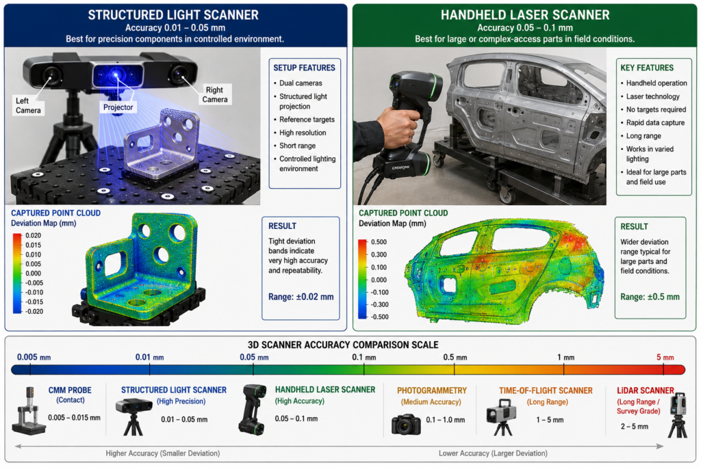
The question most engineering managers ask when considering 3D scanning for reverse engineering is not whether it produces better geometry. Most engineers accept that answer without much debate. The real question is whether it justifies the investment: the capital cost of the scanner, the software license, the training time, and the ongoing operational overhead. Does all of that add up to a lower total cost than having a skilled engineer measure the part and model it by hand?
The honest answer: it depends on part complexity, project volume, quality requirements, and whether you are building in-house capability or using a service bureau. For simple prismatic parts at low volumes, manual modeling is often cheaper. For complex organic geometry, worn legacy parts, large variant families, or regulated applications requiring measurement traceability, scan-to-CAD is typically both faster and cheaper in total cost, and qualitatively superior.
This article builds the cost model that makes that decision quantitative rather than intuitive. It maps every cost element of both approaches, builds seven scenario-specific comparisons with realistic hour and dollar estimates, identifies the crossover point at which scanning becomes economically dominant, and provides a breakeven calculator for in-house scanner investment.
What Manual Modeling Actually Costs: The Full Picture
Manual modeling for reverse engineering is deceptively simple to estimate at the surface level: an engineer measures a part and builds a CAD model. The visible cost is the engineer’s time. But the full cost includes several elements consistently overlooked in informal comparisons, producing estimates significantly lower than reality.
The Measurement Phase: More Time Than It Looks
Manual measurement of a complex mechanical part is not quick. A simple prismatic bracket with ten defined features might take 30 to 60 minutes to measure thoroughly with calipers, depth gauges, and a surface plate. A complex casting with curved surfaces, multiple angled features, and critical bore-to-bore relationships might take 4 to 8 hours of careful measurement, often requiring CMM time for spatial relationships handheld tools cannot capture reliably.
Engineers consistently underestimate measurement time for two reasons. First, the initial pass captures obvious dimensions, and subsequent CAD modeling reveals dimensions that were not initially measured, creating back-and-forth between physical part and CAD that adds 20 to 50 percent to total measurement time. Second, complex geometry requires multiple fixture setups to reach features from different orientations.
The Modeling Phase: Where Complexity Multiplies Cost
For a simple prismatic part, an experienced engineer might spend 2 to 4 hours in CAD. For a complex casting with organic geometry, rib structures, and multiple angled bosses, the same engineer might spend 20 to 40 hours, because complex geometry requires reasoning about design intent behind every measurement: which surfaces are nominally flat, which radii are standard nominal values, which surfaces are true freeform curves? Getting this wrong produces a model reproducing worn or imprecise geometry rather than original design intent.
The Hidden Cost of Manual Measurement Errors
The most significant hidden cost in manual modeling is the error rework cycle. Manual measurement introduces errors at every step: misreading a caliper, misidentifying the datum surface, transposing a recorded value. These errors propagate into the CAD model and are typically not discovered until the model is used to manufacture a part that does not fit.
The rework cost when an error reaches manufacturing includes the incorrectly manufactured part (material, machining time, setup), the schedule delay while the error is diagnosed, and potentially production downtime costs. For a machined part with a three-day lead time, a measurement error adds three to five days to the project timeline plus the full cost of the first-off part, typically $500 to $5,000 depending on material and complexity.
Manual Modeling True Cost FormulaTotal manual cost = Measurement time + CAD modeling time + Quality check time + (Error probability x Expected rework cost). The error probability and rework cost are consistently omitted from informal comparisons. For complex parts with many interrelated dimensions, a 20 to 30 percent error rate requiring significant rework is not unusual. Including probability-weighted rework typically increases true manual modeling cost by 25 to 50 percent over a best-case estimate.
What Scan-to-CAD Actually Costs: Beyond the Scanner Price Tag
The most common objection to scan-to-CAD investment is the capital cost. This is real, typically $15,000 to $80,000 for a quality structured light system, plus $3,000 to $12,000 per year for reconstruction software. But focusing on capital cost in isolation misrepresents the economics, because this cost is amortized across every part the system processes over its operational life.
Amortizing the Capital Cost
A structured light scanning system has a practical operational life of 5 to 8 years with regular calibration. Divided over 5 years, a $40,000 scanner costs $8,000 per year in capital amortization. At 100 parts per year the scanner adds $80 of capital cost per part. At 400 parts per year, it adds $20. These numbers are negligible relative to engineer labor cost for any part of moderate complexity.
Software at $6,000 to $8,000 per year adds $15 to $80 per part at the same volumes. Consumables add approximately $5 to $20 per part. Total non-labor overhead per part ranges from $40 at high volume to $180 at low volume, both well within the labor savings for anything beyond the simplest parts.
Scan-to-CAD Labor: Where the Real Savings Appear
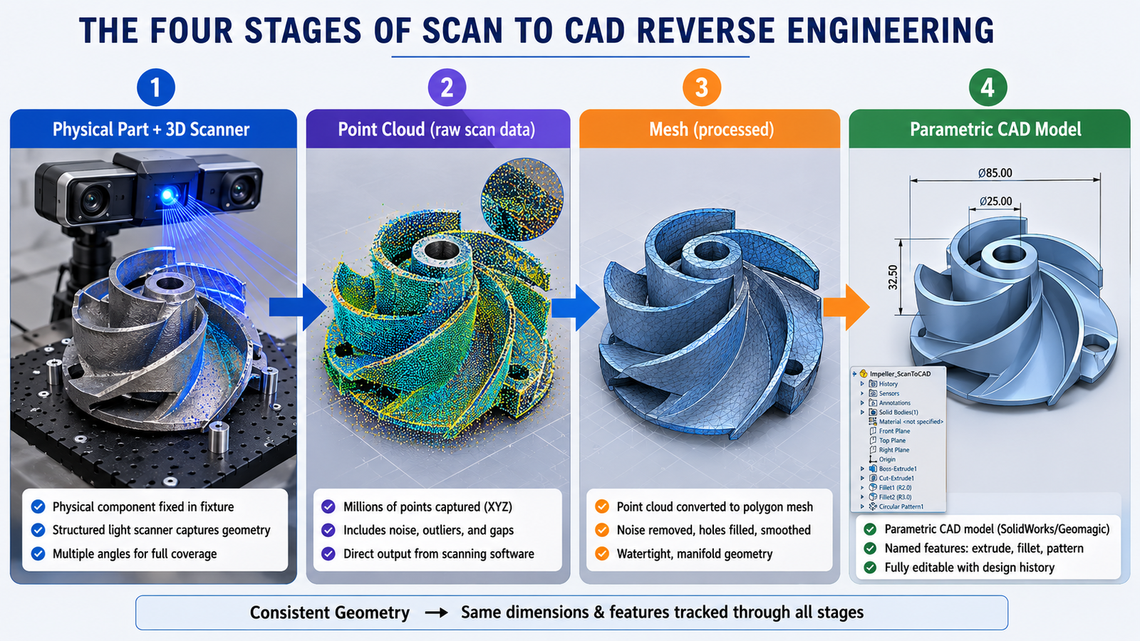
The scan capture phase typically takes 0.5 to 2 hours for a medium-sized industrial part across 6 to 15 scan positions. This compares to 1 to 8 hours of manual measurement for the same part, with the scan capturing more complete geometry without back-to-the-part re-measurement cycles.
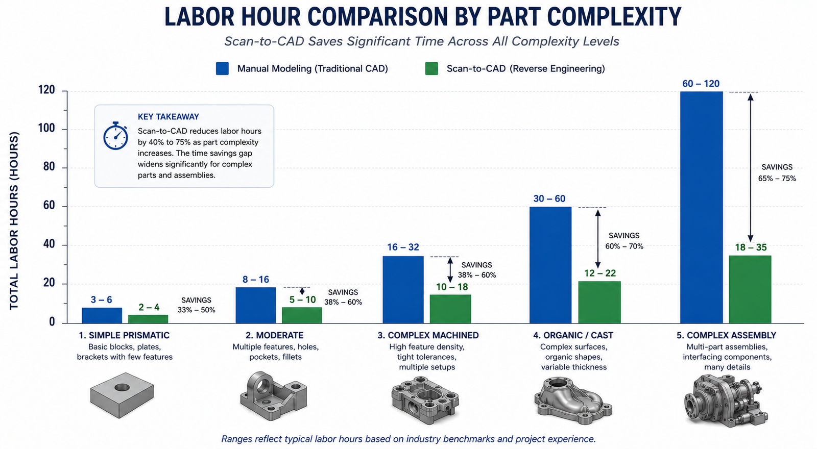
The reconstruction phase using scan-guided CAD modeling in tools like Geomagic Design X is genuinely faster than equivalent manual parametric modeling for complex geometry. For simple prismatic parts, the time saving is small. For complex castings and organic forms, scan-guided reconstruction can be 50 to 70 percent faster than equivalent manual modeling because the engineer is tracing known geometry rather than reasoning about unmeasured surfaces.
Quality Verification: The Comprehensive Advantage
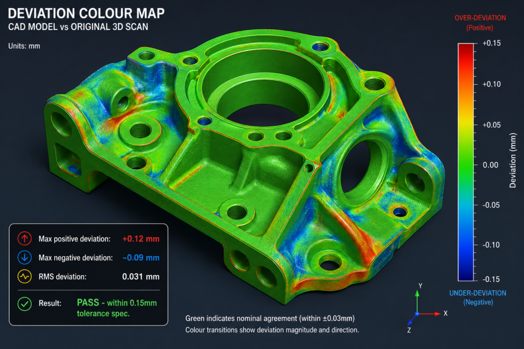
Deviation analysis, comparing the reconstructed CAD model against the original scan data, takes 1 to 3 hours for a thorough review. This has no direct equivalent in manual modeling, where verification typically means re-measuring a subset of critical dimensions. The scan verification is more comprehensive: it checks every surface simultaneously, rather than a spot-check of selected features.
This also provides a downstream asset: the scan data serves as a permanent archive of the physical geometry at the time of scanning. If questions arise months later, the scan data can be re-examined without physical access to the original part. Manual modeling produces no equivalent record.
Complete Cost Breakdown: Every Element Side by Side
The following table maps every significant cost element of both approaches with realistic ranges. All labor costs assume $100 to $150 per hour, reflecting mid-range senior engineering costs in most North American and European markets.
Scan checks entire surface; manual checks selected dimensions only
Rework risk
High – errors propagate silently to model
Low – errors visible immediately in deviation map
Manual errors typically found only at first-off manufacturing
Error rework cost (when occurs)
4-20 hrs (re-measure, re-model affected sections)
1-4 hrs (re-examine scan data, update model)
Scan data archived; no physical part access needed for re-check
Documentation package
Engineer notes only – minimal audit trail
Scan + deviation report = full traceable audit trail
Critical difference for aerospace, medical, and regulated applications
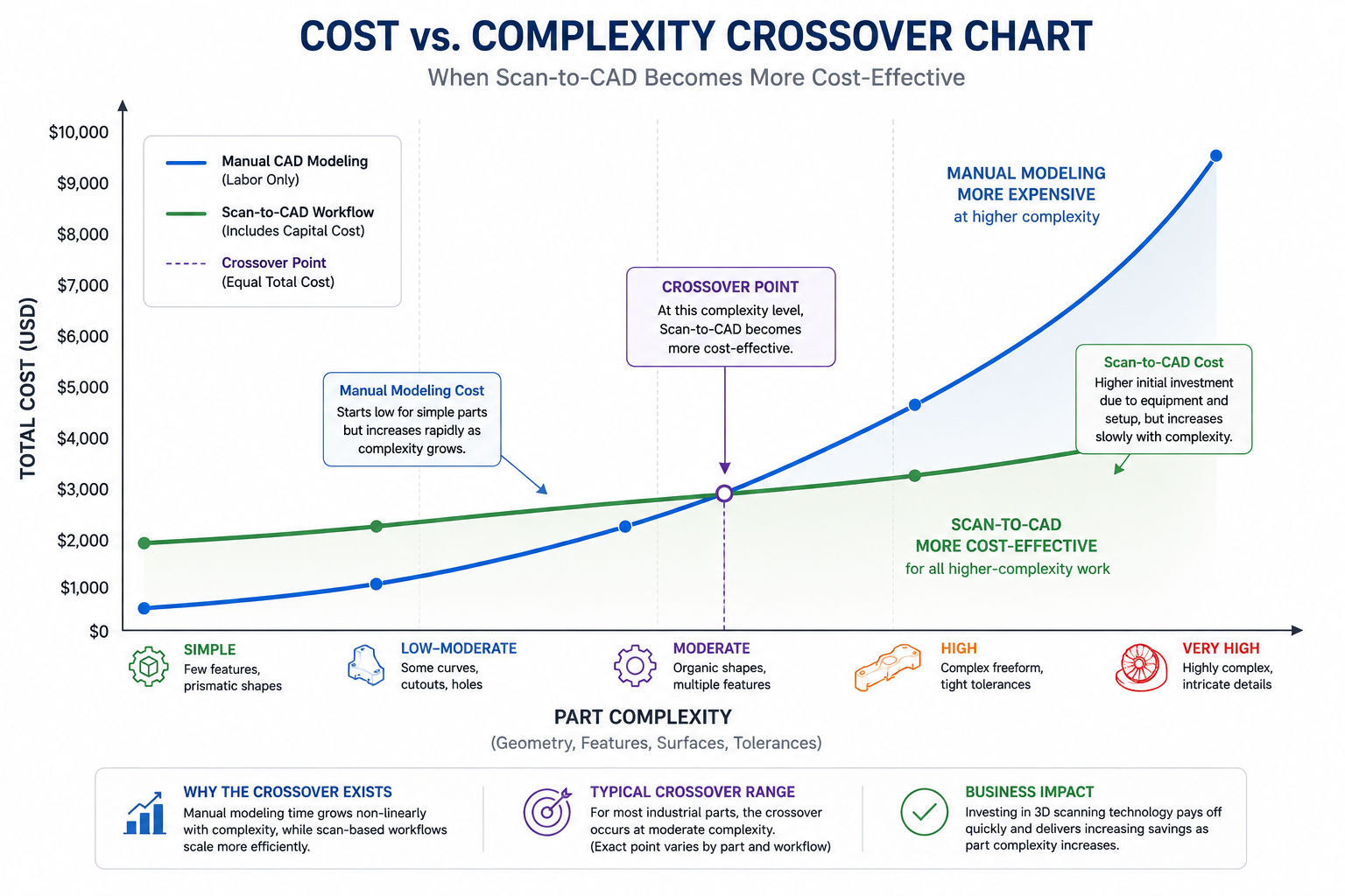
The key observation: the two approaches have similar per-part costs for simple parts but diverge dramatically as complexity increases. The scan approach’s labor time scales more slowly with complexity because the scanner captures full geometry regardless of how complex the part is, while manual measurement time scales nearly linearly with geometric complexity.
The following seven scenarios cover the range of reverse engineering situations engineering teams typically encounter, from the simplest part where manual modeling wins to the complex assembly where scanning wins decisively.
Scenario
Complexity
Manual Total
Scan-to-CAD Total
Cost Winner
Quality Winner
Simple prismatic bracket, well-documented
Low
$450-$900
$600-$1,200 (incl. scanner amortization)
Manual
Tie
Complex organic component, no drawings
High
$3,000-$9,000 (high error risk)
$1,500-$3,500
Scan-to-CAD (2-3x cheaper)
Scan-to-CAD
Worn legacy part, design intent uncertain
Med-High
$2,000-$6,000 + rework risk
$1,200-$2,500
Scan-to-CAD clearly
Scan-to-CAD
Precision machined part, H7/H6 fits
Medium
$900-$2,400
$1,400-$2,800 (CMM hybrid needed)
Tie or Manual
CMM hybrid
Family of 10 size variants
Med x10
$4,500-$9,000
$2,000-$4,000 (scan one, table for variants)
Scan-to-CAD strongly
Scan-to-CAD
Single one-off, simple geometry
Low
$300-$600
$800-$1,500 (overhead dominates)
Manual
Tie
Assembly of 15 interacting parts
High
$15,000-$45,000
$5,000-$12,000
Scan-to-CAD (3-4x cheaper)
Scan-to-CAD
The most important pattern: for simple single parts, manual wins on cost. From moderate complexity onward, and for any scenario involving multiple related parts, scan-to-CAD wins because labor savings compound while capital cost per part decreases with volume. The quality column is consistent: scanning wins for virtually every scenario beyond the simplest, because deviation analysis verifies the entire model comprehensively.
The Crossover Point: When Does Scanning Pay Off?
The crossover is a function of three variables: part complexity (determines per-part labor saving), project volume (determines capital cost amortization per part), and quality requirements (determines whether scan verification’s comprehensive documentation has additional financial value).
Complexity-Based Crossover
At 50 parts per year, scanning becomes cost-competitive at moderate complexity: roughly 20 to 50 geometric features and several organic surfaces, corresponding to approximately 10 to 20 hours of manual modeling time per part. Parts below this threshold are generally cheaper to model manually. Parts above it are almost always cheaper with scanning, often dramatically so for the most complex cases.
Volume-Based Crossover
At constant moderate complexity, each part generates roughly $500 to $1,000 in labor savings from scan-assisted modeling at $125 per hour. A $40,000 scanner with $8,000 per year software has a total annual cost of $16,000. At $750 per part average savings, the annual breakeven volume is 21 parts per year, fewer than two parts per month. This is achievable for any organization doing regular reverse engineering work. Above this volume, every additional part generates pure financial benefit.
Quality Requirement Crossover
For regulated industries, the crossover improves further because the scan verification report is a compliance asset with quantifiable financial value that reduces regulatory risk and supports quality management system audits. Including the avoided cost of alternative CMM inspection programs significantly improves scanning economics even for simpler parts in these contexts.
The Breakeven Calculator: Building Your Own Business Case
The following framework provides a structured calculation for determining the financial return on investment from a scan-to-CAD program. Adapt the numbers to your actual labor rates, scanner quotation, and part mix.
Scan-to-CAD ROI Calculator Framework
INPUTS (replace with your actual values):

  Engineer labor rate (fully loaded):         $125 / hr
  Scanner capital cost (5yr amortization):    $40,000 / 5yr = $8,000/yr
  Scan software license (annual):             $7,000 / yr
  Consumables + calibration (annual):         $1,500 / yr
  Training investment (amortized over 5yr):   $3,000 / 5yr = $600/yr

  Total annual scanning overhead:             $17,100 / yr

PER-PART ANALYSIS (adjust for your part mix):

  Average manual modeling hours per part:     18 hrs
  Average scan-to-CAD hours per part:         9 hrs
  Hours saved per part:                       9 hrs
  Labor cost saved per part:                  9 x $125 = $1,125
  Rework cost avoided (15% rate, 6hr avg):    0.15 x 6 x $125 = $112
  Total value per part:                       $1,237

BREAKEVEN VOLUME:
  Breakeven = Annual overhead / Value per part
            = $17,100 / $1,237
            = 13.8 parts/yr (round to 14)

ROI AT VARIOUS VOLUMES:
   20 parts/yr:  ($1,237 x 20)  - $17,100 =   $7,640 net annual benefit
   50 parts/yr:  ($1,237 x 50)  - $17,100 =  $44,750 net annual benefit
  100 parts/yr:  ($1,237 x 100) - $17,100 = $106,600 net annual benefit

SENSITIVITY: Simpler parts (8hr manual / 6hr scan, 2hr saving)?
  Value per part: 2hr x $125 + $112 rework avoided = $362
  Breakeven: $17,100 / $362 = 47 parts/yr (still achievable for most teams)
The most important sensitivity is the average complexity of your part mix. Teams primarily dealing with complex parts find this calculation strongly favorable even at modest volumes. Teams primarily dealing with simple prismatic parts find the breakeven higher and may be better served by accessing scanning as a service for the minority of parts that justify it.
In-House Scanning vs. Scanning as a Service
For organizations with lower volumes or highly variable project requirements, accessing 3D scanning as a service from specialist bureaus provides the quality benefits of scanning without capital investment. Understanding when each model makes sense is as important as understanding when scanning makes sense at all.
The Service Bureau Model
3D scanning service bureaus typically charge $150 to $500 per part for scan capture and mesh delivery, or $800 to $3,000 per part including full parametric reconstruction, depending on complexity and turnaround. At these rates, service bureau scanning is cost-effective for organizations doing fewer than 10 to 15 scan projects per year, or for organizations with occasional high-complexity parts within a general part mix too simple to amortize in-house equipment.
When In-House Investment Is Clearly Better
In-house scanning is the better economic choice when: the annual part volume exceeds the breakeven (typically 15 to 50 parts per year depending on complexity), when turnaround time is critical to operations, when parts are sensitive or proprietary and cannot leave the facility, or when the organization wants to develop internal scanning capability as a strategic asset. The hybrid model works well for many organizations: in-house for the majority of parts, service bureau for occasional projects requiring specialized technology.
Quality-Adjusted Cost: The Dimension Pure Cost Analysis Misses
A cost comparison looking only at labor hours and capital costs misses a genuinely important dimension: quality-adjusted cost, which accounts for the value of the quality difference between the two approaches and the cost implications of that difference over the part’s operational life.
The Verification Coverage Difference
Manual modeling produces a CAD model with spot-checked quality assurance where a subset of dimensions have been verified against the physical part. Scan-to-CAD produces a model with comprehensive surface verification through deviation analysis: every surface compared against measurement data simultaneously, rather than a spot-check of selected features.
For a replacement part that must function correctly in production equipment, a part manufactured from a spot-checked manual model carries higher residual risk of fit and function failure than one from a scan-verified model. If that residual risk materializes, the cost of the failure can easily exceed the entire cost of the original reverse engineering program.
The Documentation Value in Regulated Environments
In regulated industries, the scan data and deviation analysis report are valuable engineering documents supporting regulatory compliance, quality management system audits, and litigation defense. A manual modeling process produces essentially no documentation of the measurement process. A scan-to-CAD process produces a complete traceable chain of evidence that can be reproduced and audited years later. For pharmaceutical equipment, medical devices, aerospace components, and other regulated products, this traceability is a financial asset that reduces regulatory risk and audit response costs.
Frequently Asked Questions
Q: Is scan-to-CAD faster than manual modeling?
For complex parts, yes, significantly. For simple prismatic parts, the difference is small or nonexistent and manual modeling may be marginally faster. The time advantage grows with complexity because the scanner captures complete geometry regardless of how complex the part is, while manual measurement time scales nearly linearly. For a complex casting taking 30 to 60 hours to measure and model manually, scan-guided reconstruction typically takes 10 to 22 hours, a two to three times reduction. For a simple bracket taking 4 hours manually, scanning saves roughly 1 hour, not enough to justify scanner capital cost on a single part.
In-house structured light scanning equipment costs $15,000 to $80,000 for the scanner, plus $3,000 to $12,000 per year for professional reconstruction software. Amortized over 5 years at 50 to 100 parts per year, non-labor overhead per part is approximately $100 to $350. Scanning as a service costs $150 to $500 per part for scan capture and mesh delivery, or $800 to $3,000 per part including full parametric reconstruction, depending on complexity and turnaround requirements.
Q: What is the breakeven volume for investing in a 3D scanner for reverse engineering?
For a mid-range structured light scanner ($40,000) with professional reconstruction software ($7,000 per year) applied to moderately complex parts (15 to 20 hours manual modeling time), the typical breakeven volume is 14 to 25 parts per year. At 50 parts per year, a typical in-house scanning program generates $40,000 to $80,000 of net annual benefit beyond equipment cost.
Q: When should I use manual modeling instead of scan-to-CAD?
Manual modeling is the better choice when: the part is simple and prismatic with fewer than 10 hours of expected modeling time, project volume is too low to amortize scanner investment and service bureau pricing would exceed the manual labor cost, the part has a surviving original drawing providing complete dimensional information, or critical features are threads and precision bores requiring CMM hybrid measurement regardless of scanning approach.
Q: Does 3D scanning produce better CAD models than manual modeling?
For complex geometry, yes. Scan-to-CAD models are dimensionally referenced against comprehensive scan data throughout reconstruction, and the completed model is verified against scan data through deviation analysis. This produces a model with documented, verifiable accuracy across every surface. Manual modeling produces a model with spot-checked accuracy on selected dimensions. For simple prismatic parts, the quality difference is smaller, but the documentation advantage of scan-to-CAD remains significant for regulated applications.
Q: How do I calculate the ROI of a 3D scanner for my engineering team?
Calculate average manual modeling hours per part (measurement plus CAD plus verification plus estimated rework). Calculate expected scan-to-CAD hours per part. Multiply the difference by your fully loaded engineer labor rate to get value per part. Divide total annual scanner cost (amortized capital plus software plus consumables plus training) by value per part to get breakeven volume. If projected annual part volume exceeds breakeven, the investment is financially justified. Also include the quality value of comprehensive scan verification if your application is in a regulated industry.
Conclusion:
The cost comparison resolves into a clear framework once all relevant cost elements are accounted for. For simple parts at low volumes, manual modeling is typically cheaper because scanner overhead is not recovered from modest labor savings on straightforward geometry. For complex parts, high volumes, families of related parts, or applications with quality documentation requirements, scan-to-CAD is typically both cheaper in total cost and better in quality.
The two insights that most change how engineering managers approach this decision: first, manual modeling’s true cost includes error rework risk that is frequently omitted from informal comparisons. Second, the scan verification report is a financial asset, not just a technical product, because it reduces regulatory risk, supports quality management system audits, and provides a permanent archive proving the CAD model was correctly derived from the physical part.
Run the breakeven calculation with your own numbers. The breakeven volume for most organizations doing moderately complex reverse engineering falls at 15 to 25 parts per year, a threshold many engineering teams exceed in their first month of a serious RE program. The financial case is usually not as close as it appears before the full cost model is built.
Reverse engineering has quietly become standard practice across a far wider range of industries than most engineers realize. The image that comes to mind for most people, an aerospace engineer scanning a turbine blade or an automotive supplier benchmarking a competitor’s transmission, is accurate but represents only a fraction of where this technology now delivers value. From patient-specific orthopedic implants designed from CT scans of an individual’s anatomy, to wind farm operators scanning damaged turbine blades for repair, to museums digitizing fragile artifacts before they degrade further, reverse engineering has become a general-purpose tool for converting physical reality into usable digital design data.
What makes this article different from the lists of industries that appear elsewhere is the level of specificity. Every industry has different reasons for using reverse engineering, different accuracy requirements, different regulatory constraints, and different dominant scanning technologies. An aerospace engineer reverse engineering a structural bracket for a legacy aircraft operates under entirely different requirements than a museum conservator digitizing a sculpture, even though both processes start with a 3D scan and end with a digital model. Treating these as the same activity, as most overview content does, obscures the genuinely useful information: what does reverse engineering actually look like in your industry, specifically?
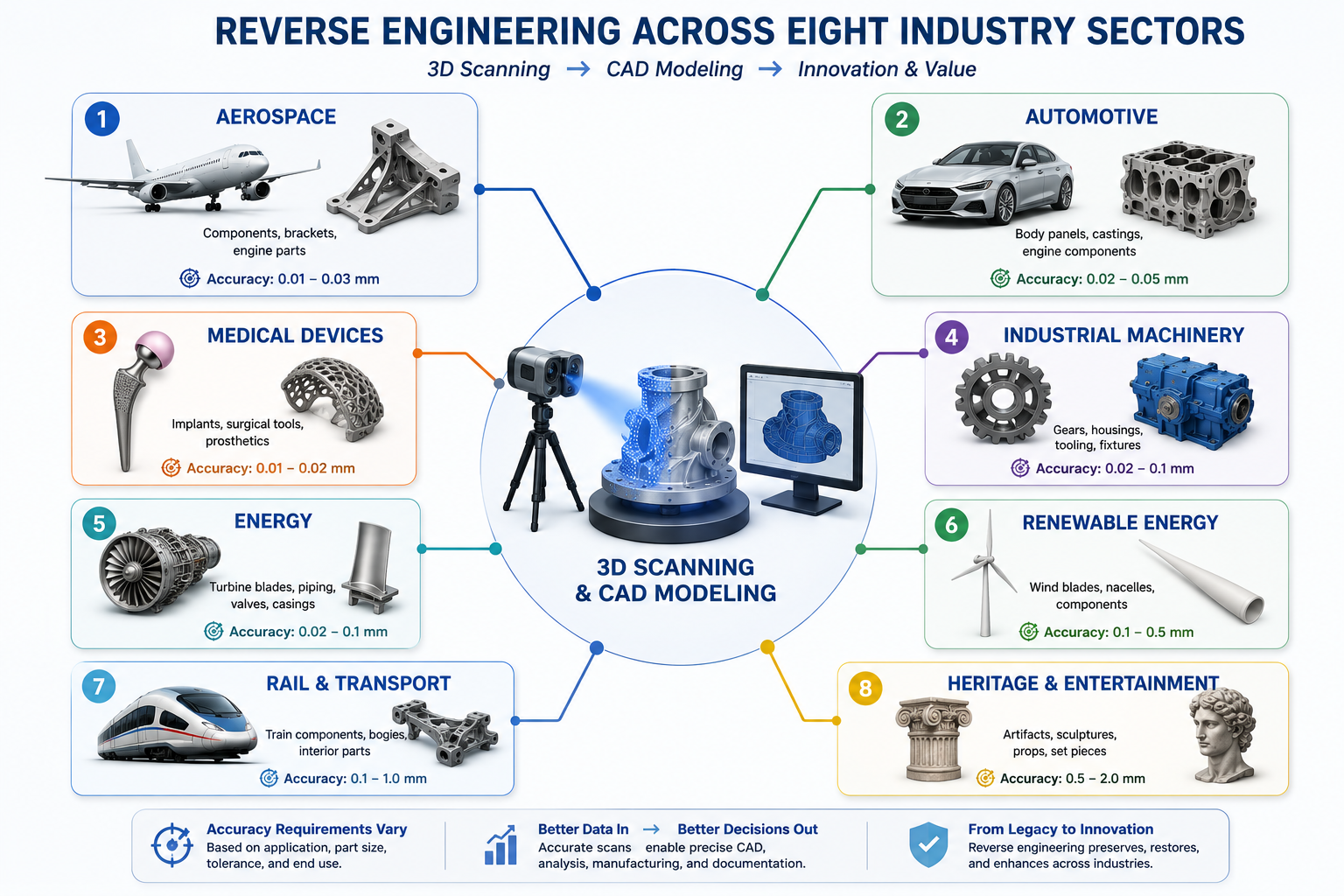
This article covers eight industry sectors where reverse engineering has become integral to operations, with the specific technical drivers, accuracy requirements, dominant technologies, and regulatory frameworks that define reverse engineering practice in each. It draws on the metrology framework and scanning technology knowledge covered in the rest of this series to explain not just that these industries use reverse engineering, but precisely how and why.
Industry Overview: Drivers, Accuracy, Technology, and Regulation
The table below summarizes the eight industries covered in this article, mapping each to its primary reverse engineering driver, typical accuracy requirement, dominant scanning technology, and the regulatory framework that governs the application. Use this as a quick reference, and refer to the detailed sections for the technical reasoning behind each entry.
Industry
Primary RE Driver
Typical Accuracy Need
Dominant Technology
Regulatory Framework
Aerospace & Defense
Legacy parts (DMSMS), OEM tooling loss
0.01 to 0.05 mm
Structured light + CMM hybrid, CT for internals
AS9100, MIL-SPEC config management
Automotive (OEM + Aftermarket)
Competitive benchmarking, legacy parts, EV development
0.02 to 0.10 mm
Structured light (ATOS), photogrammetry for large body panels
The pattern across this table reflects a consistent principle from earlier in this series: accuracy and technology requirements are driven by the application, not the industry label. Aerospace and medical devices both demand precision because of the consequences of failure, but the specific accuracy numbers and scanning technologies differ based on part geometry, material, and the specific decision the scan data will support.
1. Aerospace and Defense: Legacy Parts and DMSMS Management
Aerospace and defense represent the most mature application of reverse engineering, and the primary driver has a name that every aerospace sustainment engineer knows well: DMSMS, Diminishing Manufacturing Sources and Material Shortages. Military and commercial aircraft remain in service for 30 to 50 years or longer. The suppliers who originally manufactured specific components frequently go out of business, discontinue product lines, or lose the tooling and technical data needed to remanufacture a part long before the aircraft itself is retired.
When a part becomes unavailable through DMSMS, the operating organization faces a choice: ground the aircraft until an alternative is found, redesign the system to use a different component (an expensive and time-consuming engineering change that may require requalification), or reverse engineer the original part to enable manufacture from a new source. Reverse engineering is frequently the fastest and most cost-effective path, particularly for mechanical components, brackets, housings, and structural parts where the original design intent can be recovered reliably from the physical part.
The Aerospace Reverse Engineering Workflow
Aerospace reverse engineering follows the most rigorous version of the workflow covered earlier in this series, because the output must support airworthiness certification. The CAD model produced from the scan is not just a reference; it becomes the basis for a new technical data package that must demonstrate equivalence to the original part’s form, fit, and function. This means the deviation analysis step is not optional documentation, it is evidence submitted as part of the certification basis.
Structured light scanning combined with CMM probing for critical features is the dominant technology combination, consistent with the 10:1 measurement uncertainty ratio requirements for parts with tight tolerances. Industrial CT scanning is increasingly used for castings and complex internal geometry common in aerospace hydraulic and pneumatic components, where internal porosity assessment is also part of the material qualification process alongside geometric capture.
Configuration Management and Traceability
Every reverse engineered aerospace part must be traceable to its source data under AS9100 configuration management requirements. The scan data, the deviation analysis, the engineering judgment applied to distinguish design intent from wear (covered in detail in the previous article on scan-to-CAD challenges), and the resulting CAD model all become part of a permanent design record. This record must demonstrate that the new part is equivalent to the original in every dimension that affects form, fit, or function, with documented justification for any dimension that was idealized away from the as-scanned value.
The financial scale of this application is significant. A single grounded aircraft costs an operator tens of thousands of dollars per day in lost revenue or mission capability. A reverse engineering program that takes two weeks to produce a certified replacement part, versus a redesign and requalification process that could take a year, represents a direct and substantial cost avoidance that justifies the rigor of the aerospace reverse engineering process.
2. Automotive: Benchmarking, Legacy Parts, and EV Development
The automotive industry uses reverse engineering across three distinct applications that are often conflated in general discussions but involve different workflows and different stakeholders: competitive benchmarking, legacy and classic vehicle part reproduction, and electric vehicle development
Competitive Benchmarking
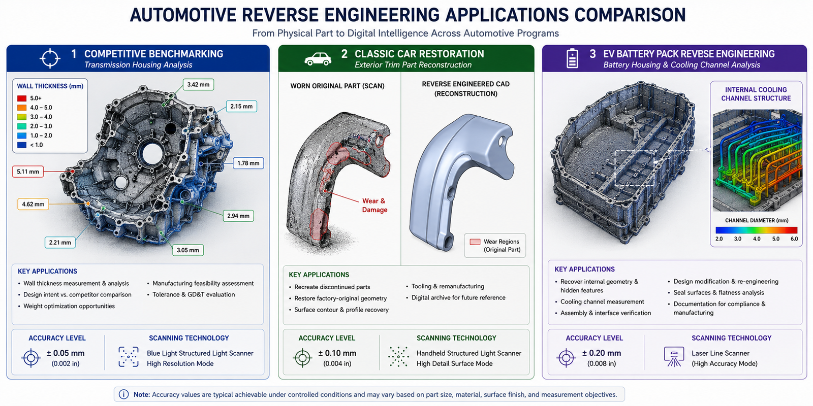
Automotive OEMs and tier-one suppliers routinely purchase competitor vehicles, disassemble them, and scan key components to understand design approaches, manufacturing methods, and material specifications. This is a legitimate and widespread practice, and it sits squarely within the legal framework for reverse engineering covered in the previous article: studying a lawfully purchased product to understand the engineering approach used by a competitor, in order to inform the design of a non-infringing alternative or to benchmark performance, is broadly protected activity in most jurisdictions.
Benchmarking scans typically focus on weight reduction opportunities (scanning a competitor’s structural component to measure wall thicknesses and rib geometry that achieve a target stiffness at lower mass), packaging efficiency (understanding how a competitor fits more functionality into a smaller volume), and manufacturing process inference (analyzing surface finish, parting lines, and feature geometry to determine whether a part is cast, forged, or machined, and what tooling approach was used). Structured light scanning with ATOS-class systems is the standard technology, providing the 0.02 to 0.05mm accuracy needed to extract meaningful wall thickness and geometry data.
Legacy and Classic Vehicle Parts
The classic car restoration market has grown into a substantial reverse engineering application in its own right. Parts for vehicles that have been out of production for decades, trim pieces, brackets, interior components, and mechanical parts, are frequently unavailable from any source. Specialist reverse engineering shops scan original parts (often the only surviving examples, sometimes in worn or damaged condition) and produce CAD models suitable for small-batch manufacturing via CNC machining, investment casting, or 3D printing.
This application directly exercises the wear-versus-design-intent challenge covered in the previous article: a 60-year-old trim part has accumulated wear, corrosion, and possibly previous repair attempts, and the reverse engineering process must distinguish what the part looked like when new from what it looks like now. The accuracy requirements are generally more relaxed than aerospace (0.1 to 0.5mm is often adequate for non-structural trim and interior parts), but the design intent recovery judgment is just as demanding.
Electric Vehicle Development
EV development has created new reverse engineering applications specific to battery and drivetrain systems. Battery pack housings, with their complex internal structures for cell modules, cooling channels, and structural support, are frequently reverse engineered during competitive analysis to understand packaging density and thermal management approaches. Drivetrain components, particularly the housings for electric motors and reduction gearboxes, are reverse engineered to support both benchmarking and the increasingly common practice of localizing manufacturing of components originally designed by a different supplier or in a different region, requiring a complete CAD redefinition from physical parts when original design data is not transferable across the supply chain relationship.
3. Medical Devices and Orthopedics: Patient-Specific Design
Medical devices represent the most technically sophisticated application of reverse engineering in this entire list, because the most advanced use case, patient-specific implant design, inverts the traditional reverse engineering workflow. Instead of scanning an existing manufactured part to recreate its design, the scan captures a patient’s individual anatomy, and the CAD model produced is an entirely new design customized to that anatomy.
Patient-Specific Implants and Surgical Guides
Orthopedic reconstruction, particularly for complex fractures, tumor resections, and revision joint replacements, increasingly uses CT scanning of the patient’s affected anatomy as the input to a design process that produces a custom implant or surgical guide matched to that individual’s bone geometry. The CT scan captures both the external bone surface and, critically, the internal trabecular bone structure and any remaining healthy bone stock after a tumor resection or in a revision surgery where previous implant material must be accommodated.
The CAD reconstruction process for these applications often references the patient’s own anatomy on the contralateral (opposite) side of the body as a mirrored design reference, applying the symmetry analysis techniques covered in the previous article, but in this case the mirrored anatomy is the design target rather than a verification check. A custom cranial implant, for example, is designed to match the mirror image of the patient’s intact skull on the opposite side, reconstructed from the CT data and verified through deviation analysis against the mirrored geometry before the implant design proceeds to manufacturing.
Legacy Device Documentation and Sustaining Engineering
Medical device manufacturers also use reverse engineering for sustaining engineering on legacy products: devices that remain on the market or in clinical use but whose original CAD data has been lost, was created in CAD software no longer supported, or belongs to a component supplier relationship that has ended. ISO 13485 and FDA 21 CFR Part 820 quality system requirements mandate that manufacturers maintain design history files for devices they support, and reverse engineering is the mechanism for reconstructing this documentation when original records are incomplete.
This application carries particular weight because medical device design changes, even changes intended only to recreate existing approved geometry, may require regulatory notification or resubmission depending on the jurisdiction and the nature of the change. The reverse engineering documentation package, including the scan data, deviation analysis, and design rationale for any idealization decisions, becomes part of the regulatory submission supporting evidence that the recreated design is equivalent to the originally approved device.
Accuracy Requirements for Medical Applications
Accuracy requirements vary significantly within medical applications. External anatomical capture for surgical planning and visualization can tolerate 0.5 to 1mm accuracy. Implant interface surfaces, the regions where the implant contacts bone or articulates with another implant component, require 0.05 to 0.1mm accuracy to ensure proper fit and function. For legacy device component reverse engineering where the device has tight manufacturing tolerances (precision mechanisms in surgical instruments, for example), the same 10:1 measurement uncertainty principles from the metrology framework apply directly.
4. Industrial Machinery and Equipment: Keeping Production Running
For manufacturing plants operating equipment that may be decades old, reverse engineering has become the primary tool for maintaining production continuity when original equipment manufacturer support has ended. This is perhaps the broadest application by sheer volume of parts: every manufacturing plant with aging equipment has wear parts, custom brackets, gearbox components, and mechanical assemblies that periodically fail and need replacement, often from OEMs that no longer exist or no longer support the specific equipment generation.
The Wear Part Reproduction Cycle
Industrial machinery reverse engineering most commonly addresses wear parts: components subject to abrasion, impact, or cyclic loading that fail predictably over time. Conveyor system components, gearbox housings, pump impellers, and custom tooling for production lines are typical examples. Because these parts fail repeatedly, plants often build a digital inventory: reverse engineer the part once, store the CAD model, and manufacture replacements on demand without needing to reverse engineer the same part again.
The wear-versus-design-intent challenge is central to this application. The part being scanned is, by definition, often a worn or partially failed example, since the failure is what triggered the need for a replacement. Engineers must distinguish the original design geometry (what the part looked like when new and functioning correctly) from the accumulated wear pattern (the geometry change that led to the failure). Reproducing the worn geometry would simply create a replacement part that fails the same way.
Custom Tooling and Fixture Reproduction
Beyond wear parts, industrial reverse engineering frequently addresses custom tooling and fixtures: jigs, gauges, and production tooling that were designed in-house or by a contract toolmaker decades ago, with no surviving CAD data. When this tooling is damaged or when a plant needs to duplicate a fixture for a second production line, scanning the existing tooling and reconstructing a CAD model is typically faster and cheaper than redesigning the fixture from functional requirements alone, particularly when the existing tooling has been refined through years of production use to address practical issues that are not documented anywhere except in the tooling’s actual geometry.
5. Energy: Oil, Gas, and Power Generation
The energy sector, encompassing oil and gas production, refining, and conventional power generation, operates some of the longest-lived capital equipment of any industry. Power generation turbines, compressors, and large valve assemblies are designed for 30 to 50 year operational lifespans, and reverse engineering has become essential for maintaining this equipment as original manufacturer support diminishes over that timeframe.
Turbine Blade Reverse Engineering
Gas and steam turbine blades are among the most demanding reverse engineering applications in any industry because they combine extremely tight aerodynamic tolerances with complex freeform organic geometry and operate in conditions that cause measurable wear and erosion over their service life. The airfoil profile of a turbine blade directly determines its aerodynamic performance, and even small deviations from the design profile measurably affect efficiency.
Reverse engineering turbine blades for repair or replacement requires structured light scanning at 0.02 to 0.05mm accuracy combined with NURBS surface reconstruction techniques (covered in the reverse engineering workflow article) to capture the complex 3D airfoil twist and camber. The wear-versus-design-intent challenge is especially significant here: blades that have been in service show erosion at the leading edge and tip, and the reconstructed CAD model must represent the original design profile, not the eroded profile, for the blade to perform correctly after repair or replacement.
Valve Bodies, Pump Casings, and Pressure Vessel Components
Large valve bodies, pump casings, and pressure vessel nozzles in process plants are frequently reverse engineered when replacement parts are needed for equipment whose original manufacturer has been acquired, merged, or gone out of business. These components often have complex internal flow passages that benefit from industrial CT scanning when the internal geometry significantly affects flow performance, combined with external structured light or laser scanning for the overall envelope and mounting interfaces.
The regulatory context for these components involves pressure equipment standards (ASME Boiler and Pressure Vessel Code, API standards for oil and gas equipment) that govern material specifications, wall thickness requirements, and pressure ratings. Reverse engineering for pressure-retaining components must verify not just geometric accuracy but also confirm that wall thicknesses meet the pressure rating requirements for the service conditions, which may require the CT-based wall thickness measurement capability covered in the previous articles.
6. Renewable Energy: Wind Turbine Blade and Component Repair
The renewable energy sector, particularly wind power, has become one of the fastest-growing applications of reverse engineering, driven by the simple economics of turbine fleet maintenance at scale. A utility-scale wind farm operator manages dozens to hundreds of turbines, each with blades that experience leading-edge erosion, lightning strike damage, and occasional structural damage from extreme weather events.
Blade Damage Assessment and Repair Design
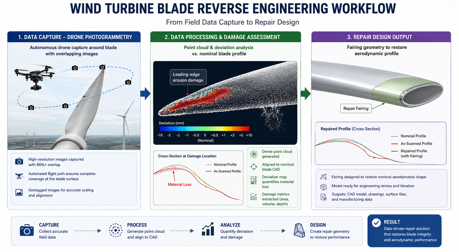
When a wind turbine blade is damaged, whether from erosion, impact, or lightning strike, drone-based photogrammetry has become the standard technology for capturing the blade’s current geometry without requiring the turbine to be taken offline for a manual inspection that would require climbing or rope access. The drone flies a defined pattern around the blade, capturing overlapping photographs that are processed into a 3D model using the photogrammetry techniques covered earlier in this series.
The accuracy requirements for blade damage assessment are more relaxed than the metrology applications discussed elsewhere, typically 0.5 to 2mm is adequate, because the primary decisions being made are whether damage exceeds repair thresholds defined by the blade manufacturer’s maintenance manual, and what repair geometry (filler material extent, aerodynamic fairing shape) is needed to restore the blade profile. This is squarely in the category of application where, as discussed in the accuracy requirements article, the required accuracy should be matched to the engineering decision being made rather than defaulting to precision metrology standards.
Gearbox and Drivetrain Component Reverse Engineering
Wind turbine gearboxes and main bearing housings represent a higher-accuracy application within the renewable sector. These components have precision-toleranced interfaces (bearing bores, gear mounting faces) that require 0.05 to 0.2mm accuracy consistent with general mechanical reverse engineering requirements. As the wind energy sector matures and the first generation of utility-scale turbines reaches the end of their original manufacturer’s support lifecycle (a similar dynamic to the DMSMS challenges in aerospace), reverse engineering of drivetrain components for fleet-wide spare parts programs is becoming increasingly common.
Solar energy applications are more limited but include reverse engineering of mounting hardware and tracking system components for older installations where the original racking manufacturer is no longer in business, a smaller-scale version of the same legacy parts dynamic seen throughout this article.
7. Rail and Heavy Transportation
Rail systems, encompassing passenger and freight rolling stock, signaling infrastructure, and track equipment, share the long-service-life characteristics of aerospace and energy equipment, with rolling stock often remaining in service for 30 to 40 years and signaling infrastructure sometimes for even longer. The reverse engineering applications in this sector closely parallel those in industrial machinery and aerospace, but with their own regulatory framework and specific component types.
Bogie and Running Gear Components
The bogie (the wheeled chassis units under a railcar) contains numerous precision mechanical components: axle boxes, suspension elements, brake system components, and coupling hardware. When these components require replacement for older rolling stock and the original manufacturer’s parts are unavailable, reverse engineering under EN 15085 (the European standard for railway vehicle welding) and equivalent regional standards governs the process for structural and safety-critical components.
Accuracy requirements for bogie components are generally in the 0.05 to 0.5mm range depending on the specific component’s function, consistent with general mechanical engineering tolerances. The structural and safety-critical nature of many rail components means that, similar to aerospace, the reverse engineering documentation package becomes part of the safety case for the component’s continued use, requiring the same rigor in distinguishing design intent from wear and damage covered throughout this series.
Signaling and Interlocking Equipment
Rail signaling equipment, much of which was installed decades ago and remains in service due to the enormous cost and operational disruption of replacing entire signaling systems, includes mechanical components, relay housings, and interface hardware that may need reverse engineering when original parts fail. This application is closer to the industrial machinery category in its accuracy requirements and workflow, but operates within rail-specific safety certification frameworks that govern any change to safety-critical signaling infrastructure.
8. Heritage, Museums, and Entertainment
The final industry in this list represents the most different application of reverse engineering from the engineering-focused applications above, but it has grown into a substantial and technically interesting field in its own right. Cultural heritage digitization, museum conservation, and entertainment production all use 3D scanning and CAD reconstruction, but the goals, accuracy requirements, and downstream uses differ significantly from manufacturing applications.
Artifact Digitization and Conservation
Museums and cultural institutions increasingly digitize their collections for multiple purposes: creating permanent digital records of fragile artifacts before they degrade further, enabling virtual access to objects that cannot be safely displayed or handled, and supporting conservation work by documenting an object’s condition at a point in time for comparison with future condition assessments. Photogrammetry and structured light scanning are both used depending on the object’s size, material, and fragility.
Accuracy requirements for heritage digitization vary enormously depending on purpose. A digital record intended for public access through a web viewer may need only 1 to 2mm accuracy, sufficient for visual fidelity. A conservation documentation project intended to detect subtle changes in an artifact’s condition over years or decades, such as monitoring crack propagation in a stone sculpture, may require sub-millimeter accuracy to reliably detect changes that are smaller than the natural variation in repeated measurements.
Entertainment: Props, Costumes, and Practical Effects
Film, television, and themed entertainment production uses reverse engineering for a different but related purpose: reproducing physical props, costume elements, and practical effects pieces at different scales, in different materials, or in multiple copies for production needs. A hero prop (the primary, screen-used version of an object) might be scanned so that stunt doubles, backup copies, or merchandise versions can be produced with consistent geometry.
This application has more relaxed accuracy requirements than virtually any other in this article, typically 0.5 to 2mm, because the output is judged by visual and tactile fidelity rather than dimensional conformance to an engineering tolerance. However, the reconstruction workflow still benefits from the parametric vs. mesh-based reconstruction decision covered in the original reverse engineering workflow article: props intended for CNC machining or 3D printing in multiple scales benefit from parametric reconstruction that can be scaled cleanly, while one-off visual reproductions may be adequately served by direct mesh output.
The Common Thread Across all eight industries, the same underlying technical framework applies: define the engineering intent before scanning, select scanning technology and accuracy appropriate to that intent (not to the most precise option available), apply the wear-versus-design-intent judgment when the scanned object has a service history, and verify the final output through deviation analysis appropriate to the application’s accuracy requirement. The industries differ in their specific drivers, regulatory frameworks, and typical accuracy targets, but the underlying engineering discipline is the same discipline covered throughout this series.
Frequently Asked Questions
Q: Which industries use reverse engineering the most?
Aerospace and defense, automotive, medical devices, industrial machinery and equipment, energy (oil, gas, and power generation), renewable energy (particularly wind power), rail and heavy transportation, and heritage/entertainment are the eight major industry sectors with established reverse engineering practices. Aerospace and defense have the longest history of formalized reverse engineering due to DMSMS (Diminishing Manufacturing Sources and Material Shortages) challenges with long-service-life aircraft. Industrial machinery represents the broadest application by volume, as every manufacturing plant with aging equipment encounters parts that need reverse engineering when original manufacturers are no longer available.
Q: What is DMSMS and why does it drive reverse engineering in aerospace?
DMSMS stands for Diminishing Manufacturing Sources and Material Shortages, a formal term used in aerospace and defense to describe the loss of suppliers, manufacturing capability, or technical data for components in long-service-life systems. Military and commercial aircraft remain in service for 30 to 50 years, far longer than the typical lifespan of the original component suppliers. When a part becomes unavailable due to DMSMS, reverse engineering is often the fastest path to producing a certified replacement, by scanning a surviving example of the part, reconstructing a CAD model, performing deviation analysis to verify accuracy, and developing a new technical data package that demonstrates equivalence to the original part for airworthiness certification.
Q: How is reverse engineering used in medical device manufacturing?
Medical device reverse engineering has two main applications. First, patient-specific implant design uses CT scanning of an individual patient’s anatomy as input to design a custom implant or surgical guide matched to that patient, often using the mirror image of the patient’s healthy contralateral anatomy as the design reference. Second, legacy device sustaining engineering reconstructs CAD models and design history documentation for devices whose original design data has been lost, required under ISO 13485 and FDA 21 CFR Part 820 quality system regulations. Accuracy requirements range from 0.5-1mm for general anatomical visualization to 0.05-0.1mm for implant interface surfaces that must fit precisely against bone or other implant components.
Q: Why do wind farms use reverse engineering for turbine blades?
Wind turbine blades experience leading-edge erosion, lightning strike damage, and occasional structural damage over their 20+ year service life. Drone-based photogrammetry has become the standard method for capturing blade geometry without requiring the turbine to be taken offline for manual rope-access inspection. The resulting 3D model is compared against the blade’s nominal design profile through deviation analysis to assess whether damage exceeds repair thresholds and to design the repair geometry (filler material, aerodynamic fairing) needed to restore the blade’s aerodynamic profile. Accuracy requirements are typically 0.5 to 2mm, matched to the repair decision rather than precision metrology standards.
Q: What accuracy is needed for industrial machinery reverse engineering?
Industrial machinery reverse engineering, primarily for wear part reproduction and custom tooling, typically requires 0.05 to 0.3mm accuracy depending on the component’s function and fit requirements. The most significant technical challenge is distinguishing the original design geometry from accumulated wear, since the part being scanned is often the worn or partially failed example that triggered the need for a replacement. Reproducing the worn geometry would create a replacement that fails the same way. This requires the wear-versus-design-intent analysis covered in scan-to-CAD conversion best practices, using evidence such as surviving unworn surfaces and manufacturing process knowledge to identify the original design dimensions.
Q: Is reverse engineering legal for automotive competitive benchmarking?
In most jurisdictions, reverse engineering a lawfully purchased competitor vehicle or component for the purpose of understanding design approaches, benchmarking performance, or informing the design of a non-infringing alternative is a legally protected activity. This is distinct from reproducing patented functionality or infringing registered trade dress, which carries legal risk regardless of how the design information was obtained. Automotive OEMs and suppliers routinely purchase and disassemble competitor vehicles for benchmarking. As with any competitive reverse engineering program, documenting the purpose clearly and consulting intellectual property counsel for programs that may result in commercial products is recommended.
Conclusion:
The eight industries covered in this article appear, at first glance, to have little in common. An aerospace sustainment engineer recreating a certified aircraft bracket, a surgeon’s engineering team designing a custom cranial implant, and a museum conservator digitizing a fragile sculpture are working in entirely different worlds, with different stakeholders, different consequences for error, and different definitions of success.
But the underlying discipline is the same. Every one of these applications starts with the same question covered at the beginning of the reverse engineering workflow article in this series: what is the engineering intent of this project, and what accuracy does that intent actually require? Every one of them benefits from the same technology selection framework, the same understanding of how accuracy, resolution, and measurement uncertainty relate to the decision being made, and the same engineering judgment required to separate original design geometry from the wear, damage, or individual variation present in the physical object being scanned.
As 3D scanning technology continues to become faster, more accessible, and more affordable, the range of industries and applications that benefit from reverse engineering will continue to expand. The engineers and organizations that get the most value from this expansion will be the ones who understand the underlying discipline well enough to apply it correctly to whatever new application comes next, rather than treating each new application as an entirely new problem to solve from scratch.
The answer to this question depends entirely on what you are going to do with the scan data. An engineer who wants to 3D scan a concept model needs a fundamentally different level of scanning accuracy from one who is reverse engineering a precision bearing bore for reproduction. An architect documenting a heritage building for visualization needs different accuracy from a quality inspector verifying whether a manufactured part meets drawing tolerances. Specifying the wrong accuracy level in either direction costs time, money, or both.
Overspecifying accuracy, choosing a scanner more precise than the application requires, means paying for a capability you will never use while adding cost, slowing the workflow, and introducing complexity. Underspecifying accuracy means your scan data cannot support the decision you need to make with it, and you discover this at the most inconvenient possible moment: when the CAD model built from the scan produces parts that do not fit, when the inspection report does not have enough measurement resolution to determine whether a part passes or fails, or when the 3D-printed prototype does not match the target geometry within the printer’s own accuracy limits.
The question therefore is not a simple one, but it is an answerable one. The answer comes from understanding three things: how engineering standards define the relationship between measurement accuracy and part tolerance, how the scanning workflow itself compounds errors from the scanner through registration through reconstruction, and what the specific accuracy requirements of each major engineering application actually are in numbers that can be compared against scanner specifications.
This article covers all three with the quantitative depth that makes the answer genuinely useful: not just which scanner type to use for which application, but why, with the metrology principles that justify the numbers and make the answer defensible in an engineering review or a metrology audit.
Accuracy, Resolution, Precision, and Repeatability: Getting the Terms Right
One of the most common and consequential errors in scanner selection is confusing accuracy with resolution or precision. These terms appear on every scanner specification sheet and are frequently used interchangeably in marketing materials, but they measure fundamentally different properties of the scanner’s performance, and choosing a scanner based on the wrong specification for your application can result in a scanner that looks impressive on paper but cannot deliver the data quality your project requires.
Term
What It Measures
What It Does NOT Measure
How to Read It on Spec Sheet
Why It Matters
Accuracy (Trueness)
How close the scan measurement is to the true value of a known reference
Consistency of repeated measurements
Single value (e.g., +/-0.03mm) or formula (e.g., 0.02mm + 0.04mm/m)
Determines whether the scanner can tell you the right answer
Precision (Repeatability)
How consistent repeated measurements of the same point are
Whether the consistent result is correct
RMS of repeated measurements on same point or surface
High precision, low accuracy = consistently wrong. Both needed.
Resolution (Point Spacing)
The distance between adjacent data points in the point cloud
The dimensional accuracy of each point’s position
Point spacing (mm) or points per mm^2
Determines smallest feature the scan can represent, not how accurate those points are
Volumetric Accuracy
How accuracy degrades as measurements are taken further from the scanner
Single-point accuracy performance
Formula: base accuracy + distance factor (e.g., 0.02 + 0.04mm/m)
Critical for large parts – scanner accurate at 0.5m may be 3x worse at 3m
Registration Accuracy
Error introduced when combining multiple scan positions into one coordinate system
Single-scan accuracy before registration
RMS registration residual in post-processing software
Often the largest error source – good scanner, poor registration = poor result
Reproducibility
Consistency when different operators or different setups measure the same part
Single-operator, single-setup consistency
Gauge R&R study output (% of tolerance consumed)
Critical for production inspection – inconsistent results mean unreliable data
Accuracy vs Resolution: The Most Commonly Confused Pair
The clearest way to understand the difference between accuracy and resolution is through an analogy. Imagine a ruler marked in 1 millimeter increments. The resolution is 1 millimeter: you can distinguish objects that differ by 1 millimeter from each other. But if the ruler was manufactured with a systematic 5 percent scale error, every measurement is wrong by 5 percent of its value. A 100 millimeter measurement reads as 105 millimeters. The resolution is 1 millimeter (you can see that difference) but the accuracy is poor (the values are systematically wrong).
In 3D scanning, a scanner with 0.05 millimeter point spacing (high resolution) and 0.3 millimeter accuracy will consistently misrepresent surface positions in ways that look precise because the dense point cloud appears detailed, but the positions themselves are systematically incorrect. A bore that is 25.000 millimeters in diameter might scan as 24.700 or 25.300 millimeters due to accuracy limitations, regardless of how many points are in the bore region. Resolution tells you how fine the detail you can see is. Accuracy tells you whether what you see is true.
Accuracy vs Precision: The High Precision, Low Accuracy Trap
A scanner can be highly repeatable, producing the same result every time it measures the same point, while being consistently wrong. This is the high precision, low accuracy condition, and it is dangerous specifically because the consistency of the results creates false confidence. If a scanner consistently measures a 50.000 millimeter bore as 49.850 millimeters across ten repeated measurements, the standard deviation of those measurements is very small (suggesting high precision), but every one of them is wrong by 0.150 millimeters.
The practical implication is that both accuracy and precision are necessary for reliable measurement. A scanner that is accurate but imprecise produces noisy data that averages to the correct value but has large point-to-point variation. A scanner that is precise but inaccurate produces clean-looking data with a systematic bias that may be mistaken for good data by engineers who do not verify against known reference standards.
Volumetric Accuracy: The Most Important Specification for Large Parts
Volumetric accuracy describes how the scanner’s accuracy changes as a function of the distance over which measurements are taken. Most structured light scanners have their stated accuracy specification for a single capture volume, typically a 300 to 500 millimeter field of view. As the scan is extended across a larger object by registering multiple capture positions together, the volumetric accuracy degrades because each registration step introduces a small alignment error that accumulates across the full measurement volume.
The volumetric accuracy of a scanner is often specified as a formula rather than a single number: for example, 0.02 mm + 0.04 mm/m. This means the base accuracy is 0.02 millimeters at any single point, and for every additional meter of scan coverage, an additional 0.04 millimeters of volumetric error accumulates. For a 500 millimeter part scanned in two positions, the volumetric accuracy is 0.02 + 0.04 times 0.5 = 0.04 millimeters total. For a 2000 millimeter structure scanned across ten positions, it is 0.02 + 0.04 times 2.0 = 0.10 millimeters.
This formula-based volumetric accuracy is why large parts are systematically harder to scan accurately than small parts, even with the same scanner. An engineer who verifies that a scanner is accurate enough for a 200 millimeter part may be surprised to find that the same scanner produces unacceptable errors when scanning a 1000 millimeter assembly, because the volumetric error at that scale exceeds the tolerance requirement.
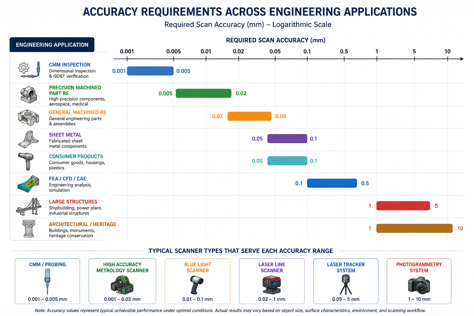
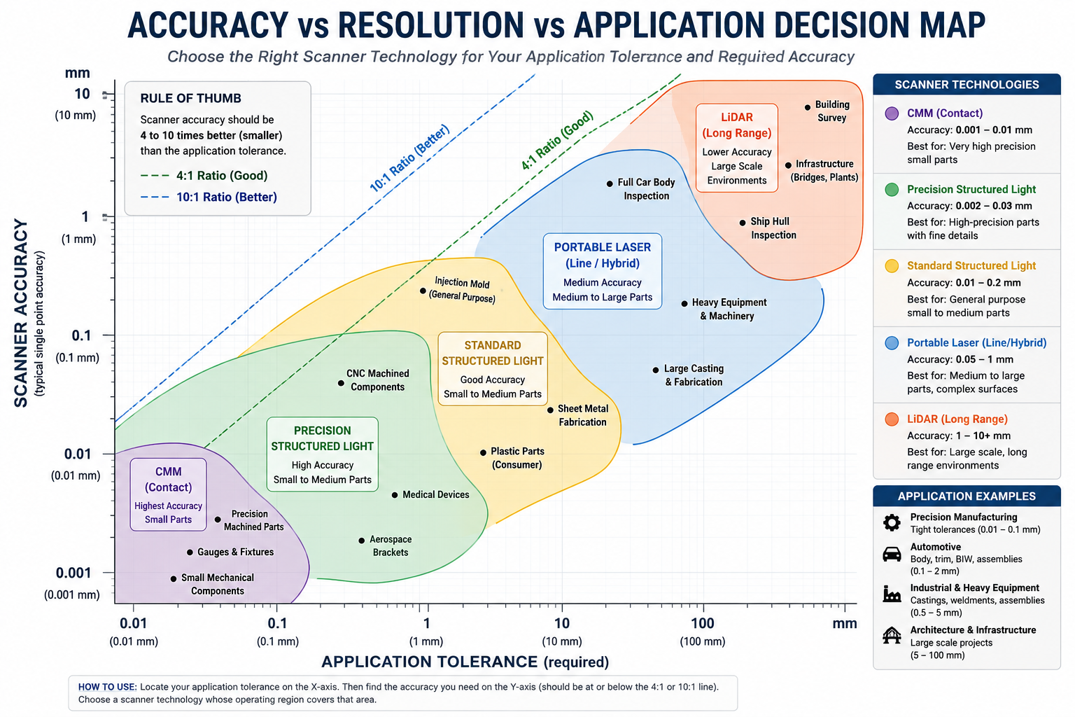
How accurate does a 3D scan need to be? As a general engineering rule, the scanner’s accuracy must be at least 4 times better than the tightest tolerance you need to verify or reproduce (the 4:1 measurement uncertainty ratio required by ASME B89 standards), and ideally 10 times better (the practical rule of thumb widely used in industry). For example: if your part has a 0.1mm tolerance, your scanner must be accurate to at least 0.025mm (4:1 rule) or ideally 0.01mm (10:1 rule). The required accuracy differs significantly by application, ranging from 0.001 to 0.005mm for precision inspection to 1 to 5mm for large structure documentation.
The 4:1 and 10:1 Measurement Uncertainty Ratios: The Mathematics Behind the Rules
When you measure a feature against a tolerance, the measurement itself introduces uncertainty. Measurement uncertainty is the range within which the true value of the measured quantity is estimated to fall, given the limitations of the measurement system. If your scanner has an accuracy of plus or minus 0.05 millimeters, a measurement that returns 10.000 millimeters means the true value is somewhere between 9.950 and 10.050 millimeters. It does not mean the true value is 10.000 millimeters.
This measurement uncertainty consumes part of the tolerance band. If the tolerance on that 10.000 millimeter dimension is plus or minus 0.10 millimeters, then the scanner’s 0.05 millimeter uncertainty consumes 50 percent of the available tolerance band. A part that actually measures 10.095 millimeters (within the 0.10 millimeter tolerance) might scan as 10.145 millimeters (outside the tolerance) due to measurement uncertainty, leading to a false rejection. A part that measures 10.105 millimeters (outside the tolerance) might scan as 10.055 millimeters (inside the tolerance), leading to a false acceptance.
The 4:1 Ratio: The ASME B89 Minimum Standard
The ASME B89 series of measurement standards and the related ASME B89.7.3.1 guidelines on measurement uncertainty establish that measurement uncertainty should not exceed one-quarter of the tolerance being verified. This is the 4:1 measurement uncertainty ratio: the measurement system uncertainty must be at least four times smaller than the tolerance. This ratio ensures that the measurement system error is small enough that false acceptance and false rejection rates are at acceptably low levels for manufacturing quality control.
Applied to 3D scanning: if your part’s tightest tolerance is 0.10 millimeters (for example, a positional tolerance on a hole pattern), your scanner’s accuracy must be 0.025 millimeters or better to meet the 4:1 ratio. This is the minimum requirement. Using a scanner with exactly this accuracy leaves only the narrowest margin for other error sources in the measurement chain (registration error, environmental effects, operator variability).
The 10:1 Ratio: The Practical Engineering Rule of Thumb
The 10:1 measurement uncertainty ratio is a more conservative target that provides adequate margin for all the error sources that exist beyond the scanner’s stated accuracy: registration error from combining multiple scan positions, mesh processing error from point cloud filtering and surface reconstruction, environmental effects from temperature variation and vibration, and operator variability from different scan setups.
The 10:1 rule says: the scanner’s accuracy should be at least ten times better than the tightest tolerance you are working with. For a 0.10 millimeter tolerance, this means 0.010 millimeter scanner accuracy. This target is more expensive to meet and may require a higher-specification scanner or a different measurement method for very tight tolerances, but it provides the measurement confidence that precision engineering decisions require.
Neither ratio is universally required by any standard. The 4:1 is the minimum established by ASME B89. The 10:1 is an engineering practice that most experienced metrologists recommend. The correct target for any specific application is determined by a formal uncertainty budget that accounts for all error sources in the specific measurement setup, not by a general rule alone. But for practical scanner selection decisions, the 10:1 rule is the safer starting point and the one that experienced engineers most consistently apply.
Building the Measurement Uncertainty Budget
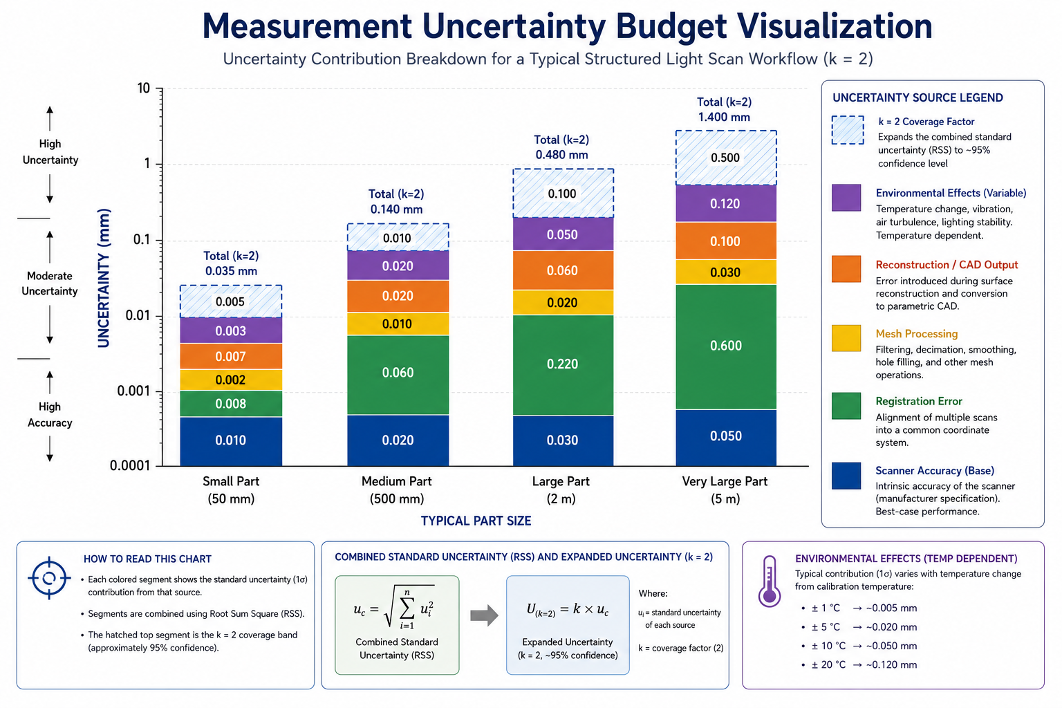
A formal measurement uncertainty budget for a scan-based measurement identifies and quantifies every source of error that contributes to the total measurement uncertainty. The individual uncertainties are combined using the root-sum-of-squares method to produce the combined measurement uncertainty. Each source contributes independently, and larger sources dominate the total.
The primary uncertainty sources in 3D scanning are:
Scanner single-scan accuracy (u1): stated by manufacturer, verified by VDI/VDE 2634 test artifact measurement
Registration error (u2): RMS residual from ICP or target-based registration of multiple scan positions
Mesh processing error (u3): error introduced by point cloud filtering, downsampling, and mesh generation
Reconstruction error (u4): error from NURBS fitting or primitive fitting in the CAD reconstruction step
Environmental error (u5): temperature variation effect (coefficient of thermal expansion times temperature uncertainty times part dimension)
Operator error (u6): variability from different setups, as quantified by gauge repeatability and reproducibility study
Combined uncertainty: U = k x sqrt(u1^2 + u2^2 + u3^2 + u4^2 + u5^2 + u6^2), where k is the coverage factor (typically 2 for 95% confidence level). The combined uncertainty U is the value that must be compared against the 4:1 or 10:1 ratio against the tolerance, not just the scanner’s stated single-scan accuracy alone.
VDI/VDE 2634 and ISO 10360: Understanding Scanner Accuracy Standards
Comparing scanner specifications across manufacturers requires understanding how each manufacturer measured and reported their accuracy. Without a common test standard, accuracy figures from different manufacturers are not directly comparable: one manufacturer might report the accuracy of their scanner measured on a flat calibration plate in controlled laboratory conditions, while another reports volumetric accuracy measured on a sphere artifact across the full working volume. Both may report similar numbers but deliver very different real-world performance.
Two standards provide the common framework for scanner accuracy testing that enables meaningful comparison.
VDI/VDE 2634: The European Standard for Optical 3D Scanners
VDI/VDE 2634 is the German guideline for the testing and characterization of optical 3D measuring systems with area sensors (the category that includes structured light scanners). Published in three parts covering point cloud and surface comparison, minimum zone fitting, and testing procedures, VDI/VDE 2634 defines specific test procedures using calibrated reference artifacts: ball bars, gauge blocks, and sphere arrays of known dimensions.
A scanner that has been tested and verified according to VDI/VDE 2634 has its accuracy measured using standardized test artifacts in defined measurement conditions. The reported accuracy figure is therefore a reproducible, verifiable measurement of the scanner’s performance rather than a manufacturer’s best-case figure from an optimized test condition. When comparing scanners, look for VDI/VDE 2634 compliance in the specification sheet. If a specification sheet does not reference the test standard used, ask the manufacturer explicitly.
VDI/VDE 2634 tests three key performance metrics: probing error (how accurately the scanner measures individual surface points on a calibrated sphere), sphere spacing error (how accurately the scanner measures distances between known reference spheres), and flatness measurement error (how accurately the scanner measures a calibrated flat surface). These three metrics together characterize the scanner’s performance for the range of measurement tasks it will encounter in practical engineering use.
ISO 10360: The International Standard for Coordinate Measuring Systems
ISO 10360 is the international standard series for acceptance testing of coordinate measuring systems, originally developed for CMMs but extended to cover optical scanning systems including laser scanners and structured light systems. ISO 10360-8 specifically covers optical distance sensors and laser scanners.
ISO 10360 tests are organized around maximum permissible errors (MPE) for length measurement, with specific test procedures using calibrated length standards (ball bars, gauge blocks) positioned throughout the scanner’s working volume. A scanner’s ISO 10360 accuracy specification is the maximum permissible error for length measurements made within its specified working volume under specified environmental conditions.
For the engineer choosing a scanner, the key practical implication of ISO 10360 is that MPE values are worst-case specifications: the scanner is guaranteed to perform no worse than the MPE in normal operating conditions. Typical performance in practice is often better than the MPE, but the MPE is what you can rely on for measurement planning. When performing a measurement uncertainty budget for a specific application, use the MPE as the scanner uncertainty input, not a claimed typical performance value that may not be reproducible in your specific conditions.
Reading a Scanner Specification Sheet Correctly
Most scanner specification sheets present multiple accuracy-related numbers that can be misleading without understanding what each represents. The following interpretation guide applies to the majority of structured light and laser scanner specifications:
“Accuracy: 0.03mm” with no further context: this is likely a best-case single-scan accuracy in optimal conditions, not volumetric accuracy across the full working distance. Ask for VDI/VDE 2634 or ISO 10360 test data.
“Resolution: 0.05mm”: this is point spacing, not accuracy. The accuracy of each point is a separate specification. High-resolution data with low accuracy is common in consumer-grade scanners marketed to the engineering community.
“Probing error: 0.025mm (VDI/VDE 2634)”: this is a meaningful, standardized accuracy specification. The probing error is the RMS deviation between scanner measurements of a calibrated sphere surface and the known sphere geometry.
“Accuracy: 0.02mm + 0.06mm/m”: this is a volumetric accuracy formula. The accuracy degrades with measurement distance as described. Calculate the expected accuracy at your specific part size using this formula before accepting it as adequate for your application.
“Repeatability: 0.01mm”: this is precision, not accuracy. It tells you the scanner will get the same answer each time, but not whether that answer is correct. Both the repeatability and the accuracy (trueness) matter.
Application-Specific Accuracy Requirements: The Numbers by Use Case
The most practical section of this article is the one that connects the metrology principles above to the specific numbers that apply to the engineering applications you are actually executing. The following table maps twelve common engineering applications to their typical part tolerance, the required scan accuracy under both the 4:1 and 10:1 ratios, and the appropriate scanner type for each.
Application
Typical Tolerance
Required Scan Accuracy (4:1 Rule)
Required Scan Accuracy (10:1 Rule)
Recommended Scanner Type
First article inspection / quality control
0.01 to 0.05 mm
0.0025 to 0.0125 mm
0.001 to 0.005 mm
CMM, or structured light with VDI/VDE 2634 certification
Precision machined part reproduction (H7/H6 fits)
0.01 to 0.02 mm
0.0025 to 0.005 mm
0.001 to 0.002 mm
CMM probing + structured light hybrid
General machined part reverse engineering
0.05 to 0.20 mm
0.0125 to 0.05 mm
0.005 to 0.02 mm
Structured light (ATOS, GOM Scan, Artec Leo)
Sheet metal and formed parts
0.10 to 0.50 mm
0.025 to 0.125 mm
0.01 to 0.05 mm
Structured light or FARO ScanArm
Injection-molded plastic consumer products
0.10 to 0.30 mm
0.025 to 0.075 mm
0.01 to 0.03 mm
Structured light or handheld laser
FEA / simulation geometry input
0.50 to 2.0 mm
0.125 to 0.5 mm
0.05 to 0.20 mm
Structured light or portable laser scanner
Additive manufacturing (FDM 0.2mm layer)
0.20 to 0.50 mm
0.05 to 0.125 mm
0.02 to 0.05 mm
Structured light or photogrammetry
Additive manufacturing (SLA 0.05mm layer)
0.05 to 0.15 mm
0.0125 to 0.0375 mm
0.005 to 0.015 mm
Structured light (precision class)
Large structure as-built documentation
1.0 to 5.0 mm
0.25 to 1.25 mm
0.10 to 0.50 mm
Laser tracker, terrestrial LiDAR
Architectural heritage / cultural preservation
0.5 to 5.0 mm
0.125 to 1.25 mm
0.05 to 0.50 mm
Terrestrial LiDAR or photogrammetry
Visual rendering / marketing 3D model
No dimensional requirement
N/A
N/A
Any scanner that produces clean mesh
Wearable / ergonomic product design
0.50 to 2.0 mm
0.125 to 0.5 mm
0.05 to 0.20 mm
Handheld structured light (Artec Leo, Eva)
Quality Control and First Article Inspection
First article inspection (FAI) is the most demanding application in the table. The measurement system must be capable of reliably determining whether a manufactured part is within the drawing tolerances, which means measurement uncertainty must be a fraction of the tolerance band. For aerospace applications where AS9102 governs first article inspection and ASME Y14.5 governs tolerances, the measurement system must demonstrate gauge repeatability and reproducibility (GR&R) of less than 10 percent of the tolerance, which is effectively the 10:1 rule expressed in GR&R terms.
For a precision-toleranced aerospace component with 0.02mm positional tolerances, achieving 10:1 ratio requires scanner accuracy of 0.002mm, which is below the performance of standard structured light systems and typically requires CMM probing for the critical features. Structured light scanning can be used for surface comparison and form deviation analysis at this tolerance level, but dimensional inspection of specific features against tight drawing tolerances generally requires CMM or CMM hybrid workflows.
Reverse Engineering for Machined Parts Reproduction
Reverse engineering for reproduction occupies the middle of the accuracy spectrum. The goal is to produce a CAD model accurate enough that parts manufactured from it fit correctly into their assembly context. For standard machined parts with H7/H6 fits (which carry tolerances of approximately 0.02mm on a 25mm bore), the 10:1 ratio requires 0.002mm scanner accuracy for the bore dimensions, again pointing to CMM hybrid measurement for the critical interfaces, with structured light providing the general surface geometry.
For general machined parts with looser tolerances of 0.1 to 0.5mm, the 10:1 ratio requires 0.01 to 0.05mm accuracy, which is well within the capability of a good-quality structured light system (0.01 to 0.05mm accuracy class). This is the sweet spot where structured light scanning delivers both speed and adequate accuracy for the application.
FEA and Simulation Geometry Input
Simulation geometry requirements are fundamentally different from inspection and reproduction requirements. The simulation result is sensitive to the boundary condition geometry, not to dimensional accuracy in the engineering tolerance sense. A fluid dynamics simulation of flow through a manifold is sensitive to the overall channel shape and cross-sectional area, not to whether the channel bore diameter is 25.000 or 25.050 millimeters. A structural FEA of a bracket is sensitive to the cross-sectional area and moment of inertia of the structural sections, not to whether a fillet radius is 3.0 or 3.1 millimeters.
This means that for simulation inputs, the accuracy requirement should be derived from a sensitivity analysis of the simulation model, not from the manufacturing tolerance of the part. A flow simulation that is insensitive to a 1mm change in channel diameter allows significantly more relaxed scan accuracy than the same channel’s manufacturing tolerance would imply. Engineers who apply manufacturing inspection accuracy standards to simulation geometry scans are overspecifying unnecessarily, adding cost and time for capability they cannot use.
Additive Manufacturing Reference Geometry
The required scan accuracy for additive manufacturing reference geometry is determined by the layer resolution of the printing process. Specifying scanner accuracy finer than the printer’s resolution provides no benefit: the printer cannot reproduce geometry at that scale regardless of how accurately the scan captured it. For FDM printing at 0.2mm layer height, scanner accuracy of 0.02 to 0.05mm is appropriate. For high-resolution SLA at 0.025mm layer height, 0.005 to 0.010mm scanner accuracy is appropriate. For metal SLS/DMLS at 0.02 to 0.05mm layer resolution, 0.005 to 0.01mm is appropriate.
The matching principle applies in both directions: overspecifying scanner accuracy wastes resources, but underspecifying means the scan data cannot support the printer’s capability. A very high-resolution resin printer scanning reference objects with a medium-quality handheld scanner will produce prints that are limited by the scan quality, not by the printer, even though the printer could produce finer detail if the reference geometry were more accurately captured.
The Accuracy Degradation Chain: How Errors Compound Through the Workflow
The scanner’s stated accuracy is only the first link in a chain of error sources that together determine the accuracy of the final CAD model produced from the scan data. Understanding this chain is essential for two reasons: it explains why the 10:1 rule is more appropriate than the 4:1 minimum for most engineering applications, and it identifies where in the workflow the most significant accuracy improvements can be made when the total error is too large for the application.
Link 1: Scanner Single-Scan Accuracy
This is the starting accuracy, the performance of the scanner within a single capture volume under optimal conditions. It is the number on the specification sheet and the one most commonly compared between scanners. For a quality structured light scanner, this is typically 0.01 to 0.05mm for industrial parts in the 100 to 500mm range.
Link 2: Registration Error
Combining multiple scan positions through ICP or target-based registration introduces alignment error at each registration step. The RMS registration residual, reported by the scan processing software after registration, quantifies this error. Typical registration residuals for a well-executed structured light scan are 0.01 to 0.05mm for ICP and 0.02 to 0.10mm for target-based registration, depending on the overlap quality and target placement.
Registration error is often the largest single contributor to total measurement uncertainty for multi-position scans of medium to large parts. An engineer who selects a scanner based on its 0.02mm single-scan accuracy but achieves only 0.08mm registration accuracy has a combined uncertainty dominated by the registration step, making the scanner’s superior single-scan accuracy irrelevant to the final result.
Link 3: Mesh Processing Error
Point cloud filtering, downsampling, and mesh generation each introduce small errors. Gaussian smoothing removes high-frequency noise but also slightly displaces surface positions from their true locations. Hole-filling algorithms estimate surface positions in regions with no scan data. Uniform downsampling replaces a cluster of points with one representative point whose position may not precisely coincide with the true surface. Collectively, these processing steps typically add 0.005 to 0.02mm of additional uncertainty to the final mesh geometry compared to the raw point cloud.
Link 4: Reconstruction Error
CAD reconstruction from the mesh introduces the fourth layer of error. Primitive fitting (fitting a mathematical plane or cylinder to a mesh region) introduces a fitting residual that depends on how well the mathematical primitive matches the actual surface. For well-formed machined surfaces, fitting residuals are typically 0.005 to 0.02mm. For less regular surfaces (cast, formed, worn), fitting residuals can be 0.05 to 0.20mm or more, as the mathematical primitive cannot accurately represent the surface’s actual non-ideal form.
NURBS surface fitting for organic geometry introduces fitting error that depends on the number of control points used. Too few control points and the surface deviates from the mesh. Too many and the surface overfits mesh noise. Typical NURBS fitting residuals for well-executed organic surface reconstruction are 0.02 to 0.10mm.
Calculating the Total Uncertainty Budget
Combining these four primary error sources using root-sum-of-squares for a typical structured light scan of a medium-sized machined part:
Example Uncertainty Budget Calculation APPLICATION: General machined part RE, target tolerance 0.10mm
UNCERTAINTY SOURCES: u1 (scanner single-scan): 0.030 mm (VDI/VDE 2634 probing error) u2 (registration): 0.040 mm (RMS residual from 6-position scan) u3 (mesh processing): 0.010 mm (after Gaussian smoothing + decimate) u4 (reconstruction): 0.015 mm (cylinder fit to bore region) u5 (thermal, 2C error): 0.005 mm (200mm aluminum, 2C temp uncertainty) u6 (operator variability): 0.015 mm (estimated from 3-setup test)
EXPANDED UNCERTAINTY (k=2, 95% confidence): U = 2 x 0.056 = 0.112 mm
CHECK AGAINST APPLICATION REQUIREMENT: 4:1 ratio requires U <= 0.10 / 4 = 0.025 mm -> FAIL (U = 0.112 mm) CONCLUSION: This workflow is NOT adequate for 0.10mm tolerance inspection. ACTION: Improve registration (tighter target placement), recalculate.
With improved registration (u2 = 0.015mm): uc = sqrt(0.0009+0.000225+0.0001+0.000225+0.000025+0.000225) = 0.038 mm U = 2 x 0.038 = 0.076 mm -> 4:1 ratio: 0.076 <= 0.025 mm -> STILL FAIL
CONCLUSION: For 0.10mm tolerance, need scanner with u1 <= 0.010mm or use CMM for critical features. Structured light adequate for form only.
This worked example demonstrates why the 10:1 rule is necessary rather than just conservative: a structured light scanner with 0.030mm stated accuracy, when used in a realistic multi-position scan workflow, produces an expanded uncertainty of 0.076 to 0.112mm. This is adequate for inspecting features with 0.50mm or looser tolerances, but it does not meet the 4:1 ratio for 0.10mm tolerances. The scanner’s stated accuracy alone would suggest it should work for 0.10mm tolerances (4:1 ratio requires 0.025mm, and 0.030mm is close). The full uncertainty budget reveals it does not.
Gauge Repeatability and Reproducibility for 3D Scanning
Gauge Repeatability and Reproducibility (GR&R) is the standard metrological method for determining whether a measurement system is adequate for a production inspection application. It has been a standard requirement in automotive quality systems (AIAG MSA) and is widely applied in ISO 9001, IATF 16949, and AS9100 quality management systems. Most engineers who work with CMMs and conventional gauges understand GR&R intuitively. Applying GR&R to 3D scanning is less common but equally important for any scanning-based inspection application that will be used to make pass-fail decisions on manufactured parts.
What a GR&R Study Measures for a 3D Scanner
A GR&R study for a 3D scanner measures how much of the total measurement variation comes from the measurement system itself versus from genuine part-to-part variation. It does this by having multiple operators scan multiple parts multiple times and analyzing the variance components: repeatability (variation within one operator’s repeated measurements of the same part), reproducibility (variation between operators’ measurements of the same part), and part-to-part variation (the genuine geometric variation between parts).
The GR&R result is typically expressed as a percentage of the tolerance: GR&R% = (measurement system variation / tolerance band) x 100%. Industry practice treats GR&R below 10% as capable (the measurement system consumes less than 10% of the tolerance band and is acceptable for production inspection), 10 to 30% as marginal (may be acceptable for some applications with management approval), and above 30% as not capable (the measurement system is consuming too much of the tolerance band to reliably distinguish conforming from nonconforming parts).
The Specific Challenges of GR&R for 3D Scanning
GR&R for 3D scanning is more complex than GR&R for contact gauges because each 3D scan measurement involves setting up the scanner, registering multiple scan positions, processing the point cloud, and extracting the dimensional result from the mesh. There are more setup variables than with a contact gauge, and each introduces its own variability.
The reproducibility component of scanning GR&R is typically larger than for CMMs because different operators may position the scanner at different distances, angles, and with different scan paths, all of which affect the data quality and the extracted dimension. For scanning-based inspection to be used in a regulated production environment, formal GR&R studies are not optional. They are the evidence that the measurement system is fit for purpose, and they identify specifically which sources of variability (operator setup, registration procedure, software settings) need to be controlled to achieve the GR&R target.
When You Do Not Need High Accuracy: Calibrating the Decision
A significant portion of 3D scanning work in engineering organizations is done at a higher accuracy level than the application requires, because the engineer defaults to the most capable scanner available or applies inspection-level accuracy standards to workflow steps that do not need them. Understanding where lower accuracy is not only acceptable but preferable saves project time and cost without compromising outcomes.
Concept Models and Form Studies
When the purpose of a scan is to capture the general shape and proportions of a physical object for reference during a design process, dimensional accuracy is almost irrelevant. A designer using a scan of an existing product as context reference for a new design needs to see the overall proportions, understand the ergonomic envelope, and reference the key interface points. Millimeter-level accuracy is more than adequate for this purpose, and a handheld consumer-grade scanner or photogrammetry from a smartphone is entirely appropriate.
Using a precision structured light scanner for this application adds cost and time for capability that never benefits the project. The scan data will not be used for inspection or reproduction. It will be used as a visual reference, and the accuracy of a 0.5mm scanner is indistinguishable from a 0.01mm scanner when the output is a reference mesh displayed on a monitor.
Large Structure Documentation
As-built documentation of buildings, facilities, and large infrastructure has very different accuracy requirements from precision part inspection. For architectural as-built documentation, 5 to 15mm accuracy is typically adequate for all design purposes: clash detection, renovation planning, MEP coordination, and general space planning. Millimeter-level accuracy is needed only for specific structural verification work or for applications that involve tight fabrication tolerances against the as-built structure.
The appropriate scanner for large structure documentation is usually a terrestrial laser scanner (LiDAR), not a structured light scanner. Terrestrial LiDAR covers the scale efficiently and achieves the 1 to 5mm accuracy that the application requires. Attempting to scan a building interior with a structured light system designed for precision mechanical parts would take weeks and thousands of scan positions without delivering meaningfully better results for the architectural application.
Simulation and FEA Geometry
As discussed in the application table, simulation geometry needs accuracy matched to the simulation’s sensitivity, not to the part’s manufacturing tolerance. Many FEA simulations are relatively insensitive to geometric accuracy at the 0.5 to 1.0mm level. A fatigue analysis of a structural weld that is insensitive to 1mm changes in the weld toe geometry does not need a scan more accurate than 0.1mm. Running a sensitivity analysis on the simulation model to determine which geometric parameters most affect the result is the correct way to determine the required scan accuracy for simulation input, rather than defaulting to the part’s manufacturing tolerance as the standard.
Practical Scanner Selection: Matching Accuracy to Application
Translating the accuracy requirements determined by the above analysis into a scanner selection decision involves matching the required accuracy (from the 4:1 or 10:1 ratio applied to the tightest tolerance) against the demonstrated accuracy of available scanner systems, verified by VDI/VDE 2634 or ISO 10360 test data rather than by unsubstantiated manufacturer claims.
The Decision Framework
Apply the following decision sequence for any new scanning application:
Identify the tightest tolerance in the application: the tightest manufacturing tolerance for inspection work, the tightest fit requirement for reproduction work, or the geometric sensitivity threshold for simulation work.
Apply the appropriate ratio: 10:1 for production inspection and precision reproduction, 4:1 minimum for lower-stakes applications where the full uncertainty budget is known and manageable.
Calculate the required accuracy: required accuracy = tolerance / ratio.
Add margin for the full uncertainty budget: if multiple scan positions will be needed (registration error) or if reconstruction will be performed (reconstruction error), add 50 to 100 percent margin to the scanner accuracy requirement to accommodate these additional error sources.
Check scanner specifications against VDI/VDE 2634 data: compare the required accuracy against the scanner’s probing error from VDI/VDE 2634 testing, not the marketing accuracy figure.
Consider volumetric accuracy at your part size: if the part is larger than the scanner’s single-capture volume, apply the volumetric accuracy formula at the expected total scan extent to verify the accuracy is still adequate at that scale.
Run a GR&R study before committing to production inspection: for any application where pass-fail decisions will be made on production parts, formally verify the measurement system’s GR&R against the tolerance before releasing the inspection method.
When to Switch Measurement Technologies
Sometimes the right answer is not a different scanner but a different measurement technology altogether. CMM probing remains superior to 3D scanning for critical dimensional inspection when the tolerances are tighter than 0.02mm, when legal traceability of individual measurement results is required, when the feature geometry is too complex for reliable scanner access (deep bores, undercut features, thread forms), or when the production rate is low enough that the speed advantage of scanning does not justify its lower accuracy.
A CMM hybrid workflow, using structured light scanning for overall surface capture and CMM probing for specific critical features, combines the coverage advantage of scanning with the accuracy advantage of probing. This is the approach described in the previous article’s treatment of thread reconstruction and is broadly applicable to any engineering metrology application where scanning alone cannot meet the accuracy requirement for all features but provides value for surface-level geometry capture.
Frequently Asked Questions
Q: How accurate does a 3D scan need to be for reverse engineering?
For reverse engineering machined parts with standard manufacturing tolerances (typically 0.05 to 0.20mm), a structured light scanner with 0.01 to 0.05mm accuracy is generally adequate. For precision-toleranced parts (H7/H6 fits, tolerances of 0.01 to 0.02mm), CMM probing for critical features is needed because structured light scanning cannot meet the 10:1 measurement uncertainty ratio at these tolerance levels. Use the 10:1 rule as a starting point: divide your tightest tolerance by 10 to get the required scanner accuracy, then verify this is achievable including the full uncertainty budget (scanner + registration + reconstruction errors combined).
Q: What is the difference between accuracy and resolution in 3D scanning?
Resolution (or point spacing) describes how densely the scanner samples the surface: the distance between adjacent measurement points in the point cloud. Accuracy describes how close each point’s measured position is to the true position of the surface at that point. A scanner can have very fine resolution (many closely spaced points) while being inaccurate (each point’s position is wrong by a significant amount). Resolution determines the smallest feature the scan can represent. Accuracy determines whether the represented geometry is dimensionally correct. For engineering applications, accuracy is almost always the more critical specification.
Q: What is volumetric accuracy in 3D scanning and why does it matter for large parts?
Volumetric accuracy describes how scanner accuracy degrades over large measurement volumes when multiple scan positions are combined. It is often expressed as a formula: base accuracy + distance-dependent error (for example, 0.02mm + 0.04mm per meter). For a 500mm part, this formula gives 0.02 + 0.02 = 0.04mm volumetric accuracy. For a 2000mm structure, it gives 0.02 + 0.08 = 0.10mm. Volumetric accuracy matters because engineers often verify scanner adequacy against part tolerances using the single-scan accuracy figure, without accounting for how accuracy degrades when the scan is extended across a larger area through multiple registered positions. Always calculate volumetric accuracy at your specific part size, not just the single-scan accuracy.
Q: What does VDI/VDE 2634 mean on a 3D scanner specification sheet?
VDI/VDE 2634 is the German guideline series for testing the accuracy of optical 3D measuring systems. When a scanner specification sheet references VDI/VDE 2634, it means the stated accuracy was measured using standardized test artifacts (calibrated spheres and ball bars) following defined test procedures. This makes the accuracy figure comparable across different manufacturers because the same test method was used. Without a VDI/VDE 2634 or ISO 10360 reference, an accuracy figure on a specification sheet may reflect only a best-case measurement in optimized laboratory conditions, not a reproducible representation of real-world performance.
Q: What is the 4:1 measurement uncertainty ratio in 3D scanning?
The 4:1 measurement uncertainty ratio is a minimum standard from ASME B89 measurement guidelines stating that a measurement system’s expanded uncertainty should be no more than one-quarter of the tolerance being verified. For 3D scanning: if your part’s tightest tolerance is 0.10mm, your scanner’s expanded uncertainty (combining scanner accuracy, registration error, mesh processing, and reconstruction errors) must be 0.025mm or better to meet the 4:1 minimum. The 10:1 ratio (0.010mm expanded uncertainty for 0.10mm tolerance) is a more conservative and widely recommended target that provides adequate margin for all practical error sources in a real scanning workflow.
Q: Do I need a GR&R study for 3D scanning inspection?
Yes, for any 3D scanning application where pass-fail decisions on production parts will be made, a formal gauge repeatability and reproducibility (GR&R) study is required by most quality management systems (AIAG MSA, IATF 16949, AS9100) to demonstrate that the measurement system is fit for purpose. A GR&R study measures the total measurement variation from the scanner and the inspection procedure (repeatability) and from different operators and setups (reproducibility), then expresses it as a percentage of the tolerance band. GR&R below 10 percent of tolerance is considered capable. Above 30 percent is considered not capable.
Q: Can I use a consumer-grade 3D scanner for engineering work?
Consumer-grade 3D scanners (including many handheld scanners marketed for hobbyist and prosumer use) typically achieve accuracy in the 0.1 to 1.0mm range. They are suitable for engineering applications that do not require precision: concept model capture, ergonomic form studies, large reference geometry, visual reference meshes for design context, and 3D printing reference geometry at FDM resolution levels. They are not suitable for inspection, precision reverse engineering for reproduction, fit-critical assembly work, or any application where tolerances are tighter than 0.5mm. Before using any scanner for an engineering application, calculate the required accuracy using the 10:1 rule and compare against the scanner’s VDI/VDE 2634 or ISO 10360 verified accuracy figure.
Conclusion:
The answer to the question this article started with, how accurate does a 3D scan need to be, is now a framework rather than a number: identify the tightest tolerance or geometric sensitivity in your application, divide by the appropriate ratio (10:1 for inspection and precision reproduction, 4:1 minimum otherwise), account for the full uncertainty budget through the workflow, and match the resulting required accuracy to a scanner with VDI/VDE 2634 or ISO 10360 verified performance at that level.
The two most expensive mistakes in scanner selection are overspecifying (paying for accuracy that the application cannot use) and underspecifying (using a scanner that cannot meet the application’s accuracy requirement, discovering this problem after the scan data has already been used to make decisions). Both mistakes are preventable with the framework above, applied before the scan project begins rather than after it has delivered ambiguous results. Accuracy specification is an engineering decision, not a purchasing default
For engineers who regularly work with scan data, developing the habit of calculating the measurement uncertainty budget for every new scanning application, rather than relying on rule-of-thumb or the scanner on hand, is one of the most durable improvements to scan-to-CAD workflow quality. The calculation takes thirty minutes the first time and five minutes for subsequent similar applications. The insight it provides, that the scanner’s stated accuracy is only part of the story, prevents the class of errors that arise from trusting specification sheets without understanding what they measure and what they do not.
The part arrived with no drawings, no CAD data, and no living engineer who knew how it was originally designed. It is a bracket that has been in production for thirty years, made from a pattern that was shaped by hand and never formally documented. It needs to be reproduced, but more than that, it needs to be redesigned for a new material and a slightly different mounting interface. Someone has to go from this physical object to a fully parametric CAD model, and they have to do it with confidence that the resulting model is accurate and that any intentional design changes are clearly distinguished from as-built deviations in the original part.
This is reverse engineering in its most demanding form, and it is far more common than the engineering community typically acknowledges. Reverse engineering from 3D scan data applies to legacy parts with no documentation, worn tooling that must be reproduced, competitive analysis of market products, digital twin creation for maintenance programs, archaeological and cultural heritage digitization, and the growing field of scan-based inspection where manufactured parts are compared against their nominal CAD models.
What these applications share is a common technical challenge: converting a physical object, measured by some form of scanning technology, into a digital representation that serves a specific downstream engineering purpose. The workflow that achieves this is neither simple nor standardized. It involves hardware selection, data capture discipline, point cloud processing, geometry reconstruction that is appropriate to the object type and the engineering intent, quality verification, and final CAD output that integrates with the team’s downstream tools.
This article covers the complete workflow from first principles, with the technical specificity that engineers actually executing this work need. It covers scanner selection with specific accuracy specifications, the pre-scan setup that determines whether the resulting data is usable, the point cloud processing steps and their specific failure modes, the critical decision between mesh-based and parametric reconstruction approaches, the NURBS surfacing techniques for organic geometry, the parametric reconstruction approach for prismatic geometry, and the deviation analysis step that verifies the final CAD model against the original scan before the model is released for any downstream use.
Defining the Reverse Engineering Intent Before Picking Up a Scanner
The single most important decision in any reverse engineering project is made before any scan data is collected: what is the engineering intent of the final output? This question determines the required scan accuracy, the appropriate reconstruction strategy, the level of parametric structure needed in the CAD model, and the quality verification criteria that define when the project is complete.
Engineers who skip this definition and go straight to scanning frequently produce scan data that is accurate enough for one purpose but insufficient for another. A mesh model that is perfectly adequate for visual reference in a product design context is completely inappropriate as input for FEA where manifold topology and surface continuity are required. A parametric model reconstructed for reproduction is built differently from a parametric model reconstructed for modification and redesign. Getting the intent wrong at the beginning guarantees rework at the end.
RE Intent
Goal
Required Output
CAD Strategy
Key Software
Accuracy Priority
Exact replica / reproduction
Reproduce a physical part with no drawings
Parametric CAD model matching as-built geometry
Measure nominal geometry, reconstruct as prismatic CAD
Geomagic Design X, PolyWorks Modeler
Highest – every dimension must match
Design intent recovery
Understand what the original engineer intended
Idealized CAD model with clean nominal geometry
Infer nominal from scan, apply design intent reasoning
Geomagic Design X + CAD platform
Medium – nominal values, not as-built deviations
As-built documentation
Document the geometry of manufactured parts as they exist
Mesh or scan-accurate surface model for records
Mesh-based output, deviation analysis against nominal
PolyWorks Inspector, Geomagic Control X
High – capture actual geometry including deviations
Modification / redesign
Modify an existing part without original CAD data
Editable parametric CAD model for downstream modification
Reconstruct with parametric features, build in design intent
Geomagic Design X, SpaceClaim, Creo
Medium – accurate enough to understand the design
FEA / simulation input
Create a CAD model for structural or fluid simulation
Manifold solid suitable for meshing, may be simplified
Mesh cleanup, simplification, defeature for analysis
Ansys SpaceClaim, Geomagic Wrap, ANSA
Medium – topology integrity more important than precision
Inspection / deviation analysis
Compare manufactured part to nominal CAD drawing
Color-coded deviation map and dimensional report
No CAD reconstruction needed – direct scan vs CAD comparison
Geomagic Control X, PolyWorks Inspector, ZEISS Inspect
Highest – sub-micron in CMM applications
The Critical Distinction: As-Built vs Design Intent
One distinction within the table above deserves special attention because it affects every subsequent workflow decision: the difference between as-built geometry and design intent geometry. As-built geometry is the actual physical form of the part as it was manufactured, including all manufacturing tolerances, wear, surface roughness, and any distortion from use or storage. Design intent geometry is the idealized form that the original engineer specified, rounded to nominal dimensions and free of manufacturing variation.
A scan always captures as-built geometry. What you do with that data depends on which type of output you need. If you need an exact reproduction of the as-built part (for a replacement part that must match a worn component), you work with the as-built geometry directly and produce a CAD model that reproduces the actual dimensions including their variation from nominal. If you need to recover the original design intent (to update an old part or use it as the basis for a new design), you use the scan data as a dimensional reference but apply engineering judgment to round dimensions to probable nominal values and reconstruct the model with clean parametric features.
This distinction is invisible in the scan data itself. It is a judgment call that the engineer makes based on understanding the project’s purpose, and it shapes every subsequent workflow decision.
What is reverse engineering in CAD? Reverse engineering in CAD is the process of creating a CAD model of a physical object that has no existing digital design data. It typically involves 3D scanning the physical object to capture its geometry as a point cloud or polygon mesh, processing and cleaning the scan data, and then reconstructing a CAD model using either mesh-based surface fitting or parametric feature reconstruction depending on the object’s geometry type and the engineering intent of the output.
Selecting the Right 3D Scanning Technology
Scanner selection is a hardware decision with direct consequences for data quality, workflow complexity, and achievable accuracy. Choosing a scanner that is less accurate than the part’s tightest tolerance means the CAD model cannot be verified against the scan with confidence. Choosing a scanner that is more capable than the part requires adds cost and complexity without benefit. The selection must match the scanner’s accuracy range, volume, and surface capture capabilities to the specific requirements of the part being scanned.
Slow, expensive, part size limited by detector, radiation
Zeiss Metrotom, Nikon XT H, Waygate Phoenix
Photogrammetry
0.05 to 0.5 mm
100 mm to 100 m+
Very large objects, site survey, archaeological, low cost
Lower accuracy, texture required, no monochrome surfaces
Agisoft Metashape, RealityCapture, OpenMVG
Time-of-flight LiDAR
2 to 20 mm
1 m to 500 m
Architectural, civil, plant survey, not precision RE
Too low accuracy for precision mechanical parts
Leica BLK360, FARO Focus, Matterport
Structured Light Scanning: The Workhorse of Industrial Reverse Engineering
Structured light scanning uses a projector to cast known patterns (typically sinusoidal fringe patterns or Gray code sequences) onto the object’s surface while one or more cameras capture the deformed pattern from different angles. The deformation of the projected pattern encodes the 3D position of every surface point within the field of view. A single structured light scan captures hundreds of thousands to millions of points simultaneously, making it significantly faster than contact or laser line methods for complex surfaces.
The dominant systems for industrial reverse engineering include the Hexagon ATOS family (the industry standard in automotive and aerospace supplier measurement), the GOM Scan systems from the same company, and the Artec range for portable scanning applications. These systems achieve accuracy in the 0.01 to 0.05 mm range for typical industrial parts, which is appropriate for most precision mechanical reverse engineering tasks except those involving tight tolerances below 0.02 mm where CMM probing is more reliable.
The practical limitation of structured light scanning is sensitivity to surface characteristics. Highly reflective surfaces (polished steel, chrome, bare aluminum) reflect the projected pattern specularly rather than diffusely, saturating the cameras and producing noisy or missing data in the reflection zone. Dark or absorptive surfaces absorb too much of the projected light, producing low contrast patterns and again noisy data. Both conditions are addressed by applying a temporary matte scanning spray, typically a white anti-glare coating that provides a diffuse surface for consistent light return and washes off after scanning without leaving residue.
Industrial CT Scanning: Capturing What Surface Scanners Cannot Reach
Industrial CT scanning (computed tomography) uses X-ray transmission through the part from multiple angles to reconstruct a three-dimensional volumetric model of both the exterior and interior geometry. It is the only scanning technology that captures internal features, hidden channels, wall thickness distributions, embedded components, and porosity without destructively sectioning the part.
The engineering applications are significant: reverse engineering a hydraulic manifold with complex internal passages, capturing the internal geometry of a casting to verify wall thickness before machining, documenting the internal structure of a composite lay-up, or identifying internal porosity in a critical structural casting. All of these require CT scanning because no surface-based technology can reach the internal geometry. Typical CT accuracy for industrial applications ranges from 0.01 to 0.05 mm depending on part size and material density, comparable to structured light scanning for external surfaces but extending to internal features that structured light cannot access.
The limitations of industrial CT are cost (CT systems range from several hundred thousand to over a million dollars and are typically accessed as a service rather than owned), scan time (a complex part may take 30 to 60 minutes to scan versus minutes for structured light), and part size limitations imposed by the X-ray detector and source geometry. Most industrial CT systems handle parts up to 400 to 600 mm in their longest dimension.
Photogrammetry: When Accuracy Requirements Are Moderate and Scale Is Large
Photogrammetry uses overlapping photographs taken from multiple angles, combined with feature-matching algorithms, to reconstruct 3D geometry. Modern photogrammetry software such as Agisoft Metashape, RealityCapture, and OpenMVG can produce dense point clouds and textured mesh models from standard camera images, making it accessible without specialized scanning hardware. Accuracy for engineering applications typically ranges from 0.05 to 0.5 mm depending on camera resolution, calibration quality, and the density of coded targets used to establish the coordinate system.
Photogrammetry is appropriate for large objects where structured light scanning would require many individual scans with complex registration: aircraft structures, vehicle body panels, architectural elements, and large tooling. For precision mechanical parts where tight dimensional accuracy is required, photogrammetry is generally not suitable as the primary measurement method, though it is often used in combination with higher-accuracy systems to extend coverage on large assemblies.
Pre-Scan Setup: The Foundation of Usable Data
The quality of the final CAD model is determined in large part by decisions made before the scanner is turned on. Pre-scan setup establishes the coordinate system for the scan, ensures the part surface is in the correct condition for data capture, and creates the reference structure that will allow multiple scan positions to be accurately combined into a single registered point cloud.
Engineers who treat pre-scan setup as a formality and jump directly to scanning produce data that requires hours of post-processing to fix problems that ten minutes of setup would have prevented. Pre-scan setup is not overhead. It is the foundation on which all subsequent data quality rests.
Establishing the Datum Reference Frame
Every reverse engineering workflow must begin by establishing a datum reference frame: the coordinate system within which all scan data will be captured and within which the final CAD model will be oriented. This is not just a convenience for the engineer. It is a technical requirement for any reverse engineering project where the resulting CAD model must mate with other components, must be verified against a drawing, or must serve as the reference for future inspection measurements.
For machined parts, the datum reference frame is typically derived from the same surfaces that were used as machining datums: the primary flat face, the secondary edge or bore, and the tertiary edge or bore that together establish the three planes of the coordinate system as defined by ASME Y14.5 datum reference frame rules. Setting up the scan to capture these datum surfaces explicitly, and aligning the scan coordinate system to them as the first processing step, ensures that every dimension extracted from the scan is expressed in the same coordinate system as the original drawing.
For organic parts without obvious machining datums, the datum reference frame must be established using coded targets: physical markers affixed to the part or surrounding fixture that provide a known coordinate reference framework. A minimum of six coded targets is required to establish a stable 3D coordinate system with overdetermined redundancy. Typically 12 to 20 targets are used on a medium-complexity part to provide robust registration and reduce the impact of any individual target that is partially obscured during a scan position.
Surface Preparation for Optimal Data Capture
Surface preparation directly determines the density and quality of scan data. The following conditions require specific preparation actions:
Reflective metal surfaces: Apply matte anti-glare scanning spray (aerosol zinc oxide or titanium dioxide based). Apply in thin, even coats from 200 to 300 mm distance. Allow 60 seconds to dry. The coating thickness should be 5 to 10 microns, negligible for most RE applications but relevant for tolerance-critical measurements.
Transparent or translucent surfaces: Apply scanning spray as above. Transparent surfaces produce no scan data because the structured light pattern passes through rather than reflecting from the surface. Translucent materials scatter the light subsurface, producing noisy and inaccurate data.
Dark or black surfaces: Apply white scanning spray. Black surfaces absorb up to 95 percent of the projected light, producing very low contrast patterns and consequently noisy or missing data in shadow areas.
Complex geometries with internal features: Plan the scan sequence to capture all surfaces before any targets are repositioned. Internal features, deep pockets, and undercuts must be scanned from specific angles. Map out which scan positions are required and in what sequence before beginning to ensure complete coverage.
Large parts requiring multiple setups: Place coded targets on the part and on a surrounding fixture board before any scanning begins. Targets must be visible from at least three different scan positions to be usable for registration. Distribute targets to cover all regions of the part including areas that will be scanned from positions without direct line of sight to other positions.
Reference Object Scanning for Scale Verification
For any reverse engineering project where absolute dimensional accuracy matters (as opposed to projects where shape is needed but not precise dimensions), scan a reference object of known dimensions alongside the part. A precision gauge block, a calibrated sphere, or a measured artifact placed in the same scan provides an independent verification of the scan system’s accuracy at the time of capture.
This reference object scan serves as the quality gate for the raw data: if the measured dimensions of the reference object from the scan match the known dimensions within the specified accuracy of the scanner, the raw data quality is confirmed. If they do not match, the scan should be repeated before any processing work begins. Discovering a scale error or systematic accuracy problem after hours of mesh processing and surface reconstruction is significantly more costly than discovering it from a reference object check before processing begins.
Point Cloud Acquisition, Registration, and Cleaning
A single scan position captures only the surfaces visible from that position. Complex parts with re-entrant geometry, deep features, or surfaces on multiple sides require multiple scan positions, each capturing a portion of the part’s surface. Combining these partial scans into a single coherent point cloud is called registration, and it is where many reverse engineering workflows first encounter serious technical problems.
Multi-Scan Registration: ICP and Target-Based Alignment
Two primary methods are used to align multiple scans into a single coordinate system. Target-based registration uses the coded targets placed on the part before scanning. Because each target’s position is captured in every scan where it is visible, and because the targets are fixed to the part, the algorithm can use the known target positions as control points to align the coordinate systems of different scan positions. Target-based registration is fast and robust when sufficient targets are visible in overlapping scans.
The Iterative Closest Point (ICP) algorithm aligns two overlapping scan positions by iteratively finding corresponding points in the overlap region and minimizing the distance between them. ICP does not require targets but requires sufficient geometric overlap between adjacent scans (typically at least 30 percent) and sufficient geometric variation in the overlap region for the algorithm to find unique correspondences. Flat surfaces with little geometric variation produce poor ICP convergence because many points in the flat region are equidistant from points in the corresponding scan, giving the algorithm ambiguous correspondence information.
In practice, most reverse engineering workflows use both methods in sequence: target-based registration establishes the initial alignment between scan positions, and ICP refinement minimizes the residual error between the overlapping point clouds after the initial alignment. The final registration error, reported as the average or maximum distance between overlapping point pairs after alignment, is the first quality metric to check: it should be below the scanner’s specified accuracy for the registration to be considered acceptable.
Point Cloud Noise Reduction and Outlier Removal
Raw point clouds from any scanner contain noise: random positional errors in individual point measurements caused by sensor noise, surface roughness, subsurface scattering, or ambient light interference. They also contain outliers: individual points that are wildly incorrect due to scanner artifacts, reflections, or measurement failures at surface edges. Both noise and outliers must be addressed before any reconstruction work begins.
Statistical outlier removal identifies points whose distance from their nearest neighbors significantly exceeds the local average and removes them as likely measurement errors. The threshold for outlier removal requires engineering judgment: too aggressive and genuine sharp features (edges, holes) are removed along with the outliers; too conservative and outliers remain and create artifacts in the processed mesh. Most professional RE software (Geomagic Wrap, PolyWorks Modeler, Artec Studio) provides automatic outlier removal with adjustable sensitivity parameters.
Gaussian smoothing reduces high-frequency noise by averaging each point’s position with a weighted average of its neighbors. The smoothing kernel size determines the spatial frequency cutoff: a small kernel removes only high-frequency noise while preserving fine surface detail; a large kernel removes both noise and legitimate surface features. For mechanical parts where sharp edges are design features, use minimal smoothing to preserve edge geometry. For organic forms where the true surface is inherently smooth, more aggressive smoothing can improve mesh quality without losing meaningful geometric information.
Managing Point Cloud Density and File Size
Raw scans from modern structured light systems may contain 5 to 50 million points for a single medium-sized part. Full multi-position scans of complex parts can produce point clouds with hundreds of millions of points. Processing, visualizing, and reconstructing geometry from data at this scale places significant demands on workstation hardware and software. Uniform downsampling reduces the point count while preserving the geometric information by selecting one representative point from each cell of a regular 3D grid overlaid on the point cloud.
The appropriate downsampling resolution depends on the geometric complexity of the part and the intended use of the data. For a complex organic form with surface detail at the 0.1 mm scale, downsampling to a uniform spacing of 0.05 to 0.1 mm preserves all relevant geometric information while reducing point count by 80 to 95 percent compared to the raw data. For a prismatic machined part where the significant geometry is at the millimeter scale, downsampling to 0.5 to 1 mm spacing is typically appropriate. The goal is the minimum point density that faithfully represents the part’s geometric features at the resolution required for the intended output.
Polygon Mesh Generation and Repair
The processed point cloud represents the surface of the part as a collection of discrete points. To create a usable geometric model, these points must be connected into a continuous surface representation. Polygon mesh generation converts the point cloud into a triangulated surface mesh where every point becomes a vertex in the mesh, and adjacent vertices are connected by edges to form triangular faces that approximate the part’s surface.
The quality of the resulting mesh depends on both the quality of the input point cloud and the algorithm used for mesh generation. The Poisson surface reconstruction algorithm, available in most professional RE software, produces watertight meshes from dense point clouds by fitting a continuous indicator function to the point data. The marching cubes algorithm, used in volumetric reconstruction tools, produces meshes directly from voxelized scan data such as CT volumes. Both algorithms produce initial meshes that require subsequent repair to address common defects.
Common Mesh Defects and Their Repair
Non-manifold edges: Edges shared by more than two triangles, or edges with no adjacent triangles on one side. These violate the topological requirement for a valid solid surface. Most mesh repair tools identify and resolve non-manifold conditions automatically, typically by removing the offending triangles and retriangulating the affected region.
Holes and gaps: Regions where the mesh is open rather than closed. These occur where the scan data was incomplete (a shadowed region, a very dark surface area, or a surface obscured by a nearby feature during scanning). Holes must be filled before the mesh can be used for most downstream operations. Hole filling algorithms range from flat cap filling (suitable for small planar holes) to curvature-driven filling (which interpolates the surface curvature from the surrounding mesh to produce a smooth, geometrically appropriate fill for complex surface holes).
Duplicate and degenerate triangles: Triangles with zero area or overlapping face pairs that occupy the same spatial position. These create geometric ambiguity and must be removed and retriangulated. Most professional software removes them automatically during an initial mesh quality analysis step.
Inverted normals: Triangles whose surface normal points inward rather than outward, producing inside-out surface regions. This typically occurs at sharp concavities where the mesh reconstruction algorithm loses track of the inside-outside orientation. Normal analysis and correction tools identify and flip inverted normals automatically in most RE software.
Mesh Optimization for Different Downstream Uses
A mesh produced directly from scan data is optimized for accuracy, not for any specific downstream use. Different downstream applications have different mesh quality requirements, and the mesh often needs to be specifically prepared for its intended use. For FEA simulation, the mesh must be manifold and watertight, with a controlled maximum triangle size appropriate for the simulation’s element size requirements. Very high-density triangular meshes from scan data often need to be decimated (simplified) to a level where the FEA solver can generate tetrahedral volume elements efficiently.
For 3D printing, the mesh must be watertight with consistent outward-facing normals, and the triangle size should be fine enough that the chord error between the mesh and the true surface is smaller than the printer’s layer resolution. For FDM printing at 0.2mm layer height, a chord tolerance of 0.02 to 0.05mm is appropriate. For SLA/SLS at finer resolution, 0.005 to 0.01mm is more appropriate.
For visualization and reference, the mesh can be significantly coarser than for manufacturing applications. A mesh decimated to 10 to 20 percent of its original triangle count often retains sufficient visual fidelity for reference purposes while loading much faster in viewing applications.
The Reconstruction Decision: Organic Geometry vs Prismatic Geometry
The most consequential workflow decision in any reverse engineering project comes after the clean mesh is established: how to reconstruct the CAD geometry from the mesh? The answer is determined by the nature of the part’s geometry, and it divides the reverse engineering workflow into two fundamentally different paths that require different software tools, different skills, and produce different types of CAD output.
Prismatic geometry consists of geometric primitives: planes, cylinders, cones, spheres, and their intersections. A machined mechanical part with flat faces, cylindrical bores, chamfers, and fillets is prismatic geometry. For prismatic parts, the correct reconstruction approach is to fit geometric primitives to the scan data, extract the nominal dimensions of those primitives, and reconstruct the part as a fully parametric CAD model using those nominal dimensions. The result is a model with flat faces, circular holes, and defined radii, that looks and behaves like a natively modeled parametric CAD part.
Organic geometry consists of freeform surfaces that cannot be described by simple geometric primitives: the flowing surface of a car fender, the ergonomic contour of a handheld tool grip, the complex surface of an impeller blade, the form of a human face. For organic parts, fitting geometric primitives to the scan data is inappropriate because the surface is genuinely freeform and cannot be accurately represented by planes and cylinders. Instead, NURBS (Non-Uniform Rational B-Spline) surfaces or subdivision surfaces are fitted to the mesh to create a smooth continuous representation of the freeform geometry.
The Mixed Reality Most real-world parts contain both prismatic and organic geometry. A consumer product housing has organic exterior surfaces for aesthetic and ergonomic reasons and prismatic interior features (boss patterns, rib structures, snap-fit features) for manufacturing. A turbine blade has a precisely defined leading-edge profile that is organic, flat root faces that are prismatic, and bolt holes that are cylindrical. Professional reverse engineering software and workflow must handle both geometry types within the same part, switching approaches surface by surface based on the geometric character of each region.
Parametric Reconstruction for Prismatic Geometry
Parametric reconstruction converts a mesh of a prismatic part into a fully featured parametric CAD model with named dimensions, logical feature order, and the ability to be modified through the CAD platform’s standard feature tools. This is the highest-value output in terms of downstream usability: the engineer who receives a parametrically reconstructed model can modify it, dimension it, create drawings from it, and derive variants from it exactly as they would with a natively designed part. The scan data becomes the measurement input, and the parametric CAD model is the engineering output.
Fitting Geometric Primitives to Scan Regions
The workflow begins by segmenting the mesh into regions that correspond to distinct geometric primitives. A plane-fitting algorithm identifies regions of the mesh that are locally flat and fits a mathematical plane through them by minimizing the least-squares distance from the mesh points to the plane. A cylinder-fitting algorithm identifies regions of the mesh that have consistent curvature in one direction (characteristic of a cylindrical surface) and fits a mathematical cylinder with a specific axis and radius.
Professional RE software like Geomagic Design X, PolyWorks Modeler, and Hexagon Xpert automate much of this segmentation and fitting, but human judgment is required to determine the boundaries between regions and to evaluate the quality of each primitive fit. The residual error of the fit (the RMS distance between the mesh points and the fitted primitive) is the quality metric: a cylinder fit with an RMS residual of 0.01 mm on a bore that needs to be accurate to 0.02 mm is acceptable. The same fit on a bore that needs to be accurate to 0.005 mm is not, and requires either higher-quality scan data or a different fitting approach.
Extracting Nominal Dimensions from Fitted Primitives
Once the geometric primitives are fitted to the scan regions, their parameters represent the as-built dimensions of the part. The fitted plane’s position represents the as-built face position. The fitted cylinder’s radius represents the as-built bore radius. The distance between two fitted planes represents the as-built wall thickness.
At this point, the engineer must apply the design intent judgment described at the beginning of the article: should the CAD model be built to the as-built dimensions from the scan, or to rounded nominal dimensions that represent the original design intent? If the bore radius fitted from the scan is 12.503 mm, is the nominal dimension 12.5 mm (an obvious rounding to a standard dimension) or is the part genuinely specified at 12.503 mm because of a non-standard design decision? The scan data alone cannot answer this question. The engineer must apply knowledge of standard dimensioning practice and engineering judgment.
For parts being reproduced exactly as-built (replacement parts, wear tooling), use the as-built dimensions from the scan directly. For parts being interpreted for design intent recovery, apply standard rounding to nominal values: round to the nearest 0.5 mm for non-critical dimensions, to the nearest 0.1 mm for moderate tolerance features, and to the nearest 0.01 mm for precision features, always verifying that the rounded nominal falls within the scan’s measurement uncertainty range.
Rebuilding the Parametric Feature Tree
The final step in parametric reconstruction is building the CAD model itself, using the extracted nominal dimensions as the driving values. This is not a copy-paste operation from the scan software to the CAD platform. It is a new parametric CAD model built from scratch, using the same CAD modeling disciplines discussed in previous articles in this series: named parameters, logical feature tree order, fully constrained sketches, and thoughtful parent-child relationships.
The scan data informs every dimension in the model, but the model is built as a proper parametric CAD part, not as a mesh-imported dumb solid. The result is a model that looks and behaves identically to a natively designed parametric part, with the critical advantage that every dimension was validated against a physical measurement rather than assumed from a nominal specification.
NURBS Surface Reconstruction for Organic Geometry
For parts with organic freeform surfaces, the parametric reconstruction approach is inappropriate because the surfaces cannot be described by geometric primitives. Instead, the workflow uses NURBS surface fitting: fitting mathematical surface patches to the mesh that capture the freeform surface shape as a smooth, continuous mathematical representation that can be used in downstream CAD operations.
Understanding NURBS Surfaces in the Context of Scan Data
NURBS (Non-Uniform Rational B-Spline) surfaces are the standard mathematical representation for freeform geometry in professional CAD systems. A NURBS surface is defined by a grid of control points, a set of knot vectors, and weight values that together define a smooth surface that passes near (but not necessarily through) the control points. The surface can be evaluated to any precision at any parametric location, making it both mathematically exact and computationally manageable.
When a NURBS surface is fitted to a mesh from scan data, the fitting algorithm positions the control points to minimize the deviation between the NURBS surface and the mesh triangles. The number of control points in the NURBS grid determines the surface’s flexibility: too few control points and the surface cannot follow the shape of the mesh precisely; too many control points and the surface overfits noise in the mesh, producing undesirable ripples and undulations. Finding the right control point density is the fundamental trade-off in NURBS surface fitting from scan data
Surface Patch Layout and G2 Continuity
Complex organic parts cannot typically be represented by a single NURBS surface patch. They require a network of surface patches that together cover the entire part surface. The quality of the result depends critically on how these patches connect at their shared edges: G0 continuity means the patches share a common boundary curve (no gap) but can meet at an angle; G1 continuity means the patches share both the boundary curve and a common tangent plane at that curve (no visible crease); G2 continuity means the patches also share the same curvature at the boundary (the highest quality connection, invisible to both the eye and to curvature analysis tools).
For engineering surfaces where the quality requirement is fit and function (an injection-molded housing where the parting line must be consistent, a casting where draft angles must be uniform), G1 continuity is typically sufficient. For Class A automotive surface work where the surface must meet the stringent visual and reflectivity quality requirements of exterior vehicle body panels, G2 continuity across all patch boundaries is mandatory. The reflection line test, which moves a linear light source across the surface and observes whether reflection lines are smooth or show kinks, detects G2 violations that are invisible to direct surface inspection.
Reconstruction Tools: Geomagic Design X and PolyWorks Modeler
Geomagic Design X (now a Hexagon product) is the industry’s most widely used dedicated reverse engineering software, combining mesh processing, automatic region segmentation, primitive fitting for prismatic geometry, NURBS surface fitting for organic geometry, and a direct export path to SolidWorks, CATIA, Creo, and Inventor with history-based parametric features. Its AutoSurface function attempts to automatically divide the mesh into patches and fit NURBS surfaces, which works well for moderately complex organic forms. For higher complexity or quality requirements, the manual patch layout tools provide full control over patch boundaries and continuity constraints.
PolyWorks Modeler from InnovMetric takes a different approach, focusing on measurement-driven reconstruction where every extracted dimension is tied back to the scan data with explicit measurement uncertainty. It is preferred in metrological applications where the reconstruction must be fully traceable to the measurement data. Its NURBS surfacing capabilities are more limited than Geomagic Design X for pure organic form work, but its dimension extraction and deviation reporting capabilities are more rigorous.
Other tools including Rhino 3D with the RhinoResurf plugin, Siemens NX with its reverse engineering extensions, and Artec Studio for photogrammetry-based reconstruction each have specific strengths that make them appropriate for different workflow scenarios. The choice of software should be driven by the geometry type of the parts typically being reversed, the CAD platform used downstream, and the level of metrological rigor required in the output.
Deviation Analysis: Verifying the CAD Model Against the Scan
Deviation analysis is the quality verification step that confirms whether the CAD model produced by the reconstruction workflow accurately represents the physical object that was scanned. It is the step that most reverse engineering tutorials mention briefly or skip entirely, and it is the step that separates a reliable reverse engineering workflow from one that produces CAD models that look correct but have not been verified against the measurement data
The principle is straightforward: the final CAD model is compared to the original scan data (either the processed point cloud or the polygon mesh) by computing the signed distance from each scan point to the nearest surface of the CAD model. Points that lie on the CAD model surface have zero deviation. Points that lie outside the CAD model surface have positive deviation. Points that lie inside (which indicates the CAD model extends beyond the physical part) have negative deviation.
Color-Coded Deviation Maps
The results of a deviation analysis are typically displayed as a color-coded deviation map overlaid on the scan data or the CAD model surface, with warm colors (yellow, orange, red) indicating regions where the CAD model does not extend far enough to match the scan (the CAD is inside the physical surface), and cool colors (cyan, blue) indicating regions where the CAD model extends beyond the scan (the CAD is outside the physical surface). Green indicates regions within the specified tolerance band.
The deviation map immediately reveals two categories of issues. Systematic deviations are regions where the CAD model consistently deviates in one direction, indicating that a dimension or surface position was incorrectly extracted or that design intent rounding produced a dimension that does not match the as-built part. These require parametric model correction. Random deviations are scattered small positive and negative values distributed throughout the surface, indicating measurement noise, surface roughness, or manufacturing variation in the scanned part. These are expected and acceptable as long as they fall within the scanner’s specified accuracy range.
Acceptable Deviation Thresholds
Setting the deviation tolerance correctly is critical for interpreting the deviation map meaningfully. The tolerance should reflect both the scanner’s measurement uncertainty and the engineering accuracy required for the specific use case.
For as-built documentation: deviation should be below the scanner’s specified accuracy (typically 0.01 to 0.05 mm for structured light). Deviations outside this band indicate reconstruction error, not scan noise.
For exact reproduction: deviation should be below the tightest manufacturing tolerance in the part. A part with H7 tolerance bores (approximately 0.02 mm tolerance on a 25 mm bore) requires reconstruction accuracy below 0.01 mm for the bore dimensions to be reliably reconstructed within tolerance.
For design intent recovery: deviation should be below the dimensional uncertainty associated with rounding to nominal. If a 12.503 mm measured dimension is rounded to 12.5 mm nominal, the resulting 0.003 mm deviation is acceptable as a rounding error. Deviation significantly larger than this indicates the rounding was incorrect.
For simulation input: overall geometric accuracy is less critical than surface quality metrics. A deviation of 0.1 to 0.5 mm may be acceptable for a fluid dynamics simulation mesh where the boundary layer thickness is orders of magnitude larger than the geometric error.
Handling Large Deviations: Diagnosis and Correction
When the deviation analysis reveals large deviations in specific regions, the diagnostic process follows a specific sequence:
Identify the deviation pattern: Is it systematic (consistent direction) or random (scattered)? Is it confined to a specific feature or distributed across the surface?
Check the scan data quality: Return to the point cloud or mesh at the location of the large deviation. Is the scan data complete and smooth in that region, or is it noisy or sparse? Noisy scan data produces large deviation values that indicate scan quality problems rather than reconstruction errors.
Re-examine the reconstruction: If scan data is good but deviation is large, the reconstruction is incorrect. Re-examine the primitive fit or surface patch in that region. The deviation map identifies exactly where the reconstruction needs correction.
Correct and re-analyze: After correcting the reconstruction, re-run the deviation analysis to confirm that the correction resolved the deviation in the target region without introducing new deviations elsewhere.
Delivering the Final CAD Model: Output Formats and Documentation
The final step of the reverse engineering workflow is delivering the reconstructed CAD model in a form that serves its intended downstream use. The output format and the documentation that accompanies it determine whether the CAD model will be trusted and used correctly by the engineers, manufacturers, or inspection teams who receive it.
Parametric CAD Output for Engineering Teams
When the reverse engineering output is a parametric CAD model for an engineering team, it should be delivered in the native format of the receiving CAD platform, not as a STEP import. A model imported from STEP is a dumb solid: it can be used for reference and for manufacturing output, but it cannot be modified parametrically. The engineering team that commissioned the reverse engineering work almost certainly needs to modify the model, which means they need the parametric version.
Software like Geomagic Design X exports parametric models directly to SolidWorks (.sldprt), CATIA (.CATPart), Creo (.prt), and Inventor (.ipt) with the feature history preserved. These exports are not always perfectly structured by the RE software’s automatic tools, so review the exported feature tree before delivery and reorganize or rename features to meet the receiving team’s CAD standards. A parametric export that follows the receiving team’s naming conventions and feature organization standards is significantly more valuable than one that uses the RE software’s default feature names.
Mesh Output for Additive Manufacturing and Simulation
When the reverse engineering output is for 3D printing or simulation, the mesh model is the appropriate output rather than a parametric CAD model. Export the mesh as STL for 3D printing applications, with the chord tolerance set appropriately for the print process as described in the CAD data translation article in this series. Export as STEP or IGES for simulation preprocessing tools that work from boundary surface geometry, or directly in the solver’s native mesh format if the RE software supports it.
For CT-derived volumetric data going to FEA, the mesh can be exported directly in formats readable by simulation preprocessors such as Ansys (.cdb), Abaqus (.inp), or as a generic STL for import into meshing tools like ANSA, HyperMesh, or ICEM CFD. The mesh quality (element size, aspect ratio, skewness) must meet the solver’s quality requirements, which typically necessitates additional mesh optimization after the RE software’s initial mesh output. Document the scan accuracy and mesh quality metrics in the delivery package so the simulation engineer knows the boundary condition accuracy of the model they are working with.
Documentation Package for Regulated Applications
In regulated industries where the reverse engineered CAD model will form part of a design record (aerospace, medical devices, automotive), the documentation package is as important as the CAD model itself. The package must include the scan method and equipment used, the scanner’s calibration certificate and last calibration date, the datum reference frame definition, the registration accuracy achieved across all scan positions, the deviation analysis results with the tolerance specification and the pass-fail status of each region, and the names of the engineer who performed the reconstruction and the reviewer who verified the deviation analysis.
This documentation converts the reverse engineered CAD model from an output of unknown provenance into a metrologically traceable engineering document. For regulatory submissions and customer audits, this traceability is what separates a usable reverse engineering result from one that must be remeasured and re-documented to meet compliance requirements.
Frequently Asked Questions
Q: What is the reverse engineering process in CAD?
The reverse engineering process in CAD is a structured workflow that converts a physical object into a digital CAD model. The process involves six main stages: defining the engineering intent (what the CAD model will be used for), selecting and setting up the appropriate 3D scanning technology, capturing the object’s geometry as a raw point cloud from multiple scan positions, processing and registering the point cloud into a clean polygon mesh, reconstructing the CAD geometry from the mesh using either parametric feature modeling for prismatic objects or NURBS surface fitting for organic objects, and verifying the final CAD model against the original scan data through deviation analysis.
Q: What is the difference between structured light scanning and laser scanning for reverse engineering?
Structured light scanning projects a pattern of light (typically sinusoidal fringes) onto the object and captures the deformed pattern with cameras to calculate 3D coordinates for hundreds of thousands of points simultaneously. It achieves accuracy in the 0.01 to 0.05 mm range and is fast for complex surfaces.
Laser line scanning uses a laser line projected across the surface while a camera captures the line position, building up a point cloud line by line as the scanner moves. Laser line scanning is more flexible for large parts and field use but typically slower and slightly less accurate than structured light for medium-sized parts. Both are suitable for most industrial reverse engineering applications. The choice depends on part size, portability requirements, and access constraints.
Q: How accurate is 3D scanning for reverse engineering?
Accuracy depends entirely on the scanning technology used. CMMs (coordinate measuring machines) achieve 0.001 to 0.005 mm accuracy but are slow and contact-based. Structured light scanners achieve 0.01 to 0.05 mm for typical industrial parts. Laser line scanners achieve 0.02 to 0.10 mm. Industrial CT scanners achieve 0.01 to 0.05 mm including internal features. Photogrammetry achieves 0.05 to 0.5 mm depending on camera resolution and setup. For precision mechanical parts requiring tolerances tighter than 0.05 mm, structured light or CMM probing is required. For reference modeling or general shape capture, structured light is the best balance of accuracy and speed.
Q: What software is used for reverse engineering CAD models from scan data?
Geomagic Design X (Hexagon) is the most widely used professional reverse engineering software, supporting both parametric reconstruction for prismatic geometry and NURBS surface fitting for organic forms, with direct export to SolidWorks, CATIA, Creo, and Inventor. PolyWorks Modeler (InnovMetric) is preferred for metrological applications requiring dimensional traceability. Artec Studio is used for photogrammetry and portable scanner workflows. Ansys SpaceClaim and Siemens NX have built-in mesh-to-CAD conversion tools. For inspection rather than modeling, Geomagic Control X and PolyWorks Inspector are the standard tools for scan-vs-nominal deviation analysis.
Deviation analysis is the quality verification step in a reverse engineering workflow that compares the completed CAD model against the original scan data to confirm that the reconstruction accurately represents the physical object. It computes the signed distance from each point in the scan to the nearest surface of the CAD model and displays the results as a color-coded map where warm colors indicate regions where the CAD model is inside the physical surface and cool colors indicate regions where the CAD model extends beyond it. Regions within tolerance appear green. Deviation analysis identifies reconstruction errors before the model is released for downstream use and provides the quality documentation required in regulated industry applications.
Q: What is the difference between as-built geometry and design intent in reverse engineering?
As-built geometry is the actual physical form of the part including all manufacturing variation, tolerances, wear, and surface roughness from use. Design intent geometry is the idealized form the original engineer specified, with dimensions rounded to nominal values and free of manufacturing variation. A 3D scan always captures as-built geometry. Whether the resulting CAD model represents as-built or design intent geometry depends on the project purpose. Exact reproduction (replacement parts) requires as-built geometry. Design reuse or modification requires design intent recovery, where the engineer applies judgment to round scan dimensions to probable nominal values. This decision must be made explicitly at the beginning of the workflow as it affects every subsequent step.
Q: Can 3D scanning capture internal features for reverse engineering?
External 3D scanners (structured light, laser line) cannot capture internal features because they require line-of-sight access to the surface being measured. Industrial CT scanning (X-ray computed tomography) is the only technology that captures internal geometry non-destructively, including hidden channels, wall thicknesses, embedded features, porosity, and internal passages. CT achieves accuracy comparable to structured light scanning (0.01 to 0.05 mm) and produces a volumetric dataset that can be segmented to extract both external and internal surface geometry. For parts with critical internal features such as hydraulic manifolds, cooling channels, or sealed cavities, industrial CT is the only option for complete reverse engineering.
Conclusion:
The reverse engineering workflow described in this article is not a mechanical copying process. At every stage, engineering judgment determines the quality and usefulness of the result: the intent definition that shapes the entire workflow, the scanner selection that sets the accuracy ceiling, the datum reference frame setup that establishes the coordinate system for all subsequent measurements, the registration quality check that validates the data before processing begins, the design intent recovery decisions that separate nominal geometry from as-built variation, and the deviation analysis thresholds that define what accurate enough means for the specific application.
Engineering teams that treat reverse engineering as a technical commodity, something any engineer can do with any scanner and any software, consistently produce CAD models that either do not meet the required accuracy, cannot be modified by the receiving team, or lack the verification documentation required by their quality management system. Reverse engineering executed as a disciplined engineering workflow produces a CAD model that is as trustworthy and as useful as one designed from scratch, with the additional assurance that every dimension has been validated against a physical measurement.
The applications for this workflow are expanding. Digital twin programs in industrial maintenance, legacy part obsolescence management in defense and aerospace, competitive benchmarking in product development, and scan-based quality inspection in production, all rely on the same foundational techniques covered in this article. As scanning technology becomes faster and more accessible, the engineering discipline of reverse engineering will become a standard capability for more teams across more industries.
The investment in learning this workflow correctly, from scanner selection through deviation analysis, pays back on every project where it replaces trial-and-error part reproduction, eliminates the cost of dimensional failures in manufactured parts, or enables a legacy design to be modified and extended rather than retired because its original CAD data is lost.
Complete your CAD engineering knowledge with our guides on CAD data translation problems, multi-body modeling techniques, master models for large projects, and parametric modeling best practices.
The engineer who has never encountered a scan-to-CAD conversion problem has not done enough scan-to-CAD conversion. The workflow looks straightforward in theory: scan the part, process the data, reconstruct the CAD model. In practice, the gap between those three steps contains ten categories of problems that each have their own technical root cause, their own detection method, and their own fix strategy. Understanding them transforms what feels like a frustrating collection of random failures into a systematic set of manageable engineering challenges.
This article exists because the previous article in this series, covering the complete reverse engineering workflow from scan to CAD model, documents what a successful workflow looks like. This article covers what happens when it does not go according to plan, which in practical engineering work is frequently. The challenges described here are not edge cases. They are the routine obstacles that every engineer executing scan-to-CAD conversion at production quality will encounter within their first ten projects.
Each challenge is covered with the specificity that makes it actionable: the underlying cause that explains why the problem occurs, the detection method that identifies it reliably (because many of these challenges are not immediately obvious), the primary fix strategy, and the alternative approaches when the primary fix is not sufficient or not applicable. The article closes with the legal and intellectual property considerations that every engineer doing competitive reverse engineering must understand, a topic that most technical content on this subject ignores entirely.
Challenge Overview: Root Cause, Detection, and Fix Strategy at a Glance
The following table maps all ten major challenge categories to their root cause, detection method, primary fix strategy, and severity classification. Use it as a quick reference when diagnosing a specific problem, and refer to the detailed section for each challenge for the full technical explanation.
Challenge
Root Cause
Detection Method
Primary Fix Strategy
Severity
Reflective and dark surface scan failure
Specular reflection or light absorption prevents pattern capture
Different materials reflect light differently within same scan
Boundary noise at material interfaces
Separate scan sessions per material, CT for embedded parts
High
CAD reconstruction quality vs mesh fidelity
Parametric reconstruction cannot capture all mesh detail
Deviation analysis of reconstructed CAD vs mesh
Hybrid approach: parametric for prismatic, NURBS for organic
Medium
Color and texture loss in geometry-only formats
STEP and IGES carry no color or texture data
Visual comparison, missing appearance data
Supplement with OBJ+MTL, VRML, or 3D PDF with texture
Low to Medium
The severity ratings reflect the impact on final CAD model quality if the challenge is not addressed: Very High challenges produce CAD models that are dimensionally incorrect and cannot be used for reproduction or manufacturing without causing failures. High challenges produce models with specific inaccurate regions. Medium challenges degrade model quality or workflow efficiency without necessarily invalidating the output.
Challenge 1: Reflective, Dark, and Transparent Surfaces
Surface optical properties are the most frequently encountered obstacle in structured light and laser line scanning, and they cause the most varied and unpredictable data quality problems. Three distinct surface conditions each create different failure modes: highly reflective surfaces, dark or absorptive surfaces, and transparent or translucent surfaces.
Reflective Surfaces: Specular Glare and Data Voids
Polished metals, chrome plating, mirror finishes, and wet surfaces create specular reflection: they reflect the scanner’s projected light pattern back at a specific angle rather than diffusing it across the field of view. When the camera is not positioned at the exact specular angle, it receives no light from that surface area and records no data. When it is near the specular angle, it receives saturated light that overwhelms the camera sensor, producing blown-out pixels with no useful fringe deformation information.
The characteristic signature of specular reflection in a point cloud is a pattern of voids surrounded by noisy data: the center of the reflection zone has no points (the camera received no return), surrounded by a fringe of noisy points (the camera received partially saturated return with corrupted fringe data). Attempting to fill these voids during mesh repair produces geometrically incorrect surfaces because the hole-filling algorithm has no scan data to work from in that region.
The primary fix is matte scanning spray: a temporary aerosol coating of white titanium dioxide or zinc oxide particles that provides a diffuse, lambertian-reflective surface for consistent light return from any camera angle. Applied correctly in 2 to 3 thin coats from 200 to 300mm distance, the coating is 5 to 15 microns thick and dries to a matte white finish that the scanner reads easily. For most mechanical engineering applications, this coating thickness is negligible relative to part tolerances. For precision surface measurements where the coating thickness matters, use the thinnest possible application and account for the coating thickness in your dimensional analysis.
A secondary approach is to adjust the scanner’s exposure settings to reduce sensitivity and capture less of the saturated reflection, or to reposition the scanner to avoid the specular angle for the most problematic surfaces. Most professional scanning systems allow per-scan exposure adjustment, and some support automatic multi-exposure capture (HDR scanning) that takes multiple exposures in the same position and combines the best data from each, effectively handling mixed reflectivity across a complex surface in a single capture.
Dark and Black Surfaces: Light Absorption
Dark surfaces, particularly matte black coatings, anodized aluminum, carbon fiber, and black rubber, absorb 80 to 95 percent of incident light. The scanner’s projected pattern reaches the surface but the reflected intensity is too low for the camera to detect reliable fringe deformation. The result is sparse, noisy point data rather than complete voids, because some light does return but the signal-to-noise ratio is too low for accurate position calculation.
The fix is the same matte scanning spray, which converts the dark surface to a diffuse white reflector. For parts where spray cannot be used (due to temperature sensitivity, chemical incompatibility, or requirement for an absolutely uncoated surface), alternative approaches include increasing the scanner’s projector intensity (if the system supports it), increasing exposure time, or switching to a laser line scanner rather than a structured light system, as laser line scanners are generally less sensitive to surface color than white-light structured light systems.
Transparent and Translucent Surfaces: Subsurface Scattering
Transparent materials (glass, clear acrylic, polycarbonate lenses) transmit the scanner’s light pattern rather than reflecting it, producing no data at all from the surface. Translucent materials (frosted plastic, skin, some composites) allow light to penetrate the surface and scatter within the material before returning, a phenomenon called subsurface scattering. This produces surface data that is systematically displaced from the true surface position by the scattering depth, typically 0.1 to 2 mm depending on material type and thickness.
Scanning spray converts transparent surfaces to opaque reflectors, resolving both problems. For parts where transparency is a functional property that must be preserved (optical components, light pipes, lenses), CT scanning is the only practical alternative for capturing the surface geometry without any surface preparation.
Surface Preparation Quick Reference Polished steel, chrome, aluminum mirror finish: 2 to 3 coats matte scanning spray. Anodized aluminum, black paint, carbon fiber: 2 to 3 coats matte scanning spray. Clear glass, polycarbonate, acrylic: 2 to 3 coats matte scanning spray (destroys transparency – use CT if optical function must be preserved). Rubber or silicone: Spray carefully – rubber can absorb spray solvent. Test on an inconspicuous area first. Alternative: use blue LED structured light rather than white LED for better rubber surface response.
Challenge 2: Inaccessible Geometry and Scan Shadows
Optical scanners, including structured light, laser line, and photogrammetry systems, share an absolute limitation: they can only capture surfaces they can see. Every feature that is occluded, recessed, or hidden behind another surface during scanning creates a scan shadow: a region of the point cloud with no data because no scan position had line-of-sight access to that surface.
Common examples include the interior of deep pockets, undercut features, the back face of a flange, the interior of a tube or bore, and the region under an overhang. In complex assemblies, adjacent components shadow each other, leaving interface surfaces without scan coverage.
Multi-Position Scanning to Minimize Shadows
The primary strategy for managing scan shadows is systematic multi-position scanning: planning the scan sequence so that every surface receives at least one scan position with acceptable line-of-sight access, even if that position is geometrically difficult to achieve. Before beginning any scan session on a complex part, walk around the part and identify every surface that will be difficult to access optically. Then plan the scanner positions, fixture orientations, and part repositioning steps needed to capture each of those surfaces.
For deep pockets and internal channels, scan from inside the pocket with the scanner tilted to the maximum possible angle. Most structured light systems capture data reliably at angles up to 45 degrees from the surface normal. Beyond this angle, the projected pattern becomes too foreshortened for accurate fringe deformation measurement, and data quality degrades rapidly. Laser line scanners generally have wider acceptance angles and can capture data at 60 to 70 degrees from normal in some configurations.
Industrial CT for Enclosed Internal Geometry
When optical scanning cannot capture required internal geometry regardless of the number of scan positions, industrial CT scanning is the definitive solution. CT sees through the material from all angles simultaneously, capturing internal surfaces, channels, wall thicknesses, and enclosed features that no optical scanner can reach. For hydraulic manifolds, castings with complex internal passages, sealed housings, and any assembly with interior surfaces that define function, CT is not an optional alternative to optical scanning. It is the only technology that captures the complete geometry.
The practical limitation is that CT requires access to a CT system (either in-house or as a service), it is slower than optical scanning, and it has part size constraints. For engineering teams that regularly reverse engineer complex internal geometry, CT scanning as a service from an industrial metrology provider is a practical and cost-effective solution for the cases where optical scanning cannot reach the needed surfaces.
Reconstructing Inaccessible Geometry by Inference
When CT scanning is not available and scan shadows cannot be eliminated through multi-position scanning, the engineer must reconstruct the unseen geometry by inference: using the surrounding scan data to determine what the hidden geometry must be, based on engineering knowledge, visual reference images, or measured cross-sections.
For features that follow predictable manufacturing patterns (a drilled and tapped hole that continues through to a visible back surface, a groove that follows a radius consistent with the cutter diameter visible in the surrounding material, a blind bore whose depth can be estimated from the visible part thickness minus a minimum wall thickness), reasoned reconstruction produces reliable results. For truly arbitrary hidden geometry with no inferential constraints, the CAD model must document the unknown region explicitly in its drawing annotations and inspection requirements.
Challenge 3: Part Deformation During Scanning
Part deformation during scanning is the most damaging challenge in the list because it is invisible in the scan data. The scanner captures the geometry of the part as it actually is during the scan, including any deformation caused by its own weight, by the fixture holding it, or by the thermal environment. The resulting CAD model accurately represents the deformed part, not the part’s true geometry, and the engineer may not discover the problem until a manufactured replacement using the CAD model does not fit correctly.
Gravity Sag in Large or Flexible Parts
Gravity sag is a common deformation mode for large parts, thin flexible sheets, rubber and elastomer components, and any part where the ratio of part mass to stiffness is high enough that measurable deflection occurs under self-weight. A long, thin aluminum extrusion lying horizontally will sag at its center. A rubber seal gasket deforms significantly under its own weight if unsupported. Even a relatively stiff steel bracket can show 50 to 200 microns of sag at its free end when cantilevered, which exceeds the accuracy of a high-quality structured light scan and would produce measurable dimensional error in the resulting CAD model.
The fix is fixture design: supporting the part in a way that replicates its functional configuration, or in a way that eliminates all gravity-induced deflection. For a part that is normally bolted flat to a surface, scan it in that bolted configuration with the mounting surface as the primary datum. For a part whose functional configuration cannot be determined, scan it from multiple orientations and compare the results to identify any gravity-dependent deformation in the data.
Fixture-Induced Stress
Fixtures that clamp or constrain a flexible part to hold it for scanning introduce their own deformation. The clamping force distorts the part geometry in the clamped region and can induce bending or twisting throughout the part. This is particularly problematic for thin-walled plastic parts, sheet metal, and rubber or silicone components. Fixture-induced deformation can be worse than unconstrained gravity sag if the fixture is not designed carefully.
Use the minimum clamping force required to hold the part stable during scanning. For very flexible parts, consider non-contact fixturing: a conformal nest made from foam or sand that supports the part across its full surface without applying point or line loads. For parts where any deformation is unacceptable, use gravity-independent measurement methods: CMM probing with the part in its functional installation configuration, or CT scanning where the part can be scanned while resting naturally without clamping.
Thermal Deformation
Temperature differences between the scan environment and the part’s functional operating temperature cause dimensional changes through thermal expansion. For a 200mm aluminum part (coefficient of thermal expansion approximately 23 microns per millimeter per degree Celsius), a 10 degree Celsius temperature difference between the scan environment and the nominal temperature produces 46 microns of dimensional change, which exceeds the measurement tolerance for precision features.
Ensure the part is at thermal equilibrium with the scan environment before scanning begins. For a part that has been transported from a cold or hot environment, allow 30 to 60 minutes of equilibration time before scanning. For precision work, record the ambient temperature during scanning and apply a thermal expansion correction to the scan data if the scanning temperature differs from the reference temperature (typically 20 degrees Celsius for engineering dimensional measurement per ISO 1 standard).
Deformation Risk Assessment Low risk: Rigid metal parts under 300mm, wall thickness over 5mm, scanned in ambient conditions. Medium risk: Parts over 500mm, thin-walled structures under 3mm, machined from stock (residual stress). High risk: Rubber/elastomer parts, flexible plastics, large sheet metal, assembled multi-material parts, parts transported from extreme temperatures. For High risk parts: design a dedicated scanning fixture, verify deformation by comparing scans in two different orientations, and consult a metrology engineer before committing the scan data to a CAD reconstruction.
Challenge 4: Distinguishing Wear and Damage from Original Geometry
This is the most engineering-intensive challenge in the entire scan-to-CAD conversion process because it cannot be resolved by any software tool or measurement technique alone. It requires engineering judgment informed by multiple lines of evidence, and getting it wrong produces a CAD model that faithfully reproduces a damaged part rather than the original design.
The specific problem: the scanned part has been in service and has accumulated geometric changes from in-service wear, impact damage, corrosion, plastic deformation, or fatigue-related distortion. The scan accurately captures the current state of the part, but the reverse engineering goal is typically to reproduce the original design geometry, not the worn state. The scan data alone cannot tell you what is original design geometry and what is accumulated damage.
Types of Geometric Change from Service Life
Abrasive wear produces gradual, smooth reduction in material at contact surfaces. It is typically most severe at sliding interfaces, sealing surfaces, and bearing surfaces. In a scan, worn surfaces appear as slight concavities or reduced thicknesses relative to the expected nominal geometry. Wear patterns are often asymmetric (one side wears faster than the other due to loading direction) and have a smooth, gradual boundary with unworn regions.
Impact damage produces local depressions, cracks, or material loss at specific locations from point loading events. These are typically more localized than wear and have sharper boundaries between damaged and undamaged regions. Impact damage can produce significant local deformations: a 20mm dent in a steel plate from a dropped tool can represent 2 to 5mm of surface displacement.
Corrosion produces surface texture changes and material loss at chemically active surfaces. Early-stage corrosion produces a roughening of the surface texture that increases scan noise without significant dimensional change. Advanced corrosion produces measurable material loss and surface pitting that significantly corrupts the scan data in affected regions.
Plastic deformation from overloading produces permanent geometric change throughout the affected region. Unlike wear (which only removes material from contact surfaces) or impact damage (which is localized), plastic deformation can alter the geometry of large regions of the part in ways that are difficult to identify from the scan alone without reference to the original design dimensions.
Strategies for Identifying Wear and Damage
Use multiple evidence sources in combination to identify which geometric deviations are wear and which are original design features:
Compare to surviving unworn regions: Most worn parts have some surfaces that were not in contact with anything during service and remain at or near the original geometry. Comparing the worn surfaces to these reference regions establishes what the original dimensions likely were.
Statistical analysis of the point cloud: Wear and damage produce localized outlier deviations from the general surface geometry. Fitting a geometric primitive to the entire surface and examining the residual deviation distribution identifies regions where the deviation is anomalously large, indicating either damage or an intentional geometric feature. Large, localized positive deviations suggest material buildup or deformation. Large, localized negative deviations suggest wear or removal.
Multiple part comparison: If more than one example of the same part is available, scanning multiple examples and comparing them isolates genuine design geometry (consistent across all parts) from wear and damage (variable between parts depending on service history).
Physical reference standards: Assembly drawings, inspection sheets, or supplier part numbers from the original program may establish nominal dimensions against which the scan can be compared, identifying the magnitude and location of all deviations from nominal.
Manufacturing process inference: An engineer familiar with the manufacturing process for the part type can identify which surfaces would have been machined to a precise nominal and which would have been cast or formed with greater variation. Machined surfaces in an unworn state should have scan residuals close to the scanner’s measurement uncertainty. Larger residuals on machined surfaces indicate either wear or damage.
Challenge 5: The Symmetry Assumption Trap
The symmetry assumption trap is a specific error pattern that is extremely common among engineers who are new to scan-to-CAD conversion and surprisingly persistent among experienced ones. It occurs when an engineer, modeling a part that appears symmetric from visual inspection, applies symmetry in the CAD reconstruction without verifying from the scan data whether the part is actually symmetric within measurement precision. The result is a CAD model that is more symmetric than the physical part, which can cause fit errors in asymmetric assembly interfaces and incorrect mass properties.
Most manufactured parts that are nominally symmetric are not perfectly symmetric in their as-built state. Casting, forging, and injection molding processes all introduce manufacturing variation that is rarely perfectly symmetric. In-service loading can induce asymmetric wear or deformation. And some parts that appear symmetric actually have subtle intentional asymmetry that serves a functional purpose, such as a poka-yoke feature that prevents incorrect installation.
Detecting Asymmetry in Scan Data
The detection method is a mirror comparison analysis: reflect the scan data about the presumed plane of symmetry and compute the deviation between the original data and its mirror image. If the part is truly symmetric within the measurement uncertainty of the scanner, the deviation between original and mirror should be uniformly distributed at or below the scanner’s noise level. If specific regions show systematic deviation above the noise level, those regions are genuinely asymmetric.
Most professional scan processing software (Geomagic, PolyWorks, ZEISS Inspect) includes symmetry analysis tools that perform this comparison automatically and display the results as a color map. This analysis should be performed before any symmetry is applied in the CAD reconstruction, and its results should be documented in the project record.
The Right Response to Detected Asymmetry
When the symmetry analysis reveals asymmetry, the engineer must determine whether it represents manufacturing variation that should be idealized away or intentional design asymmetry that must be preserved. Manufacturing variation is typically random in distribution and magnitude, with no consistent directionality. Intentional design asymmetry is typically consistent across multiple examples of the same part and associated with a functional interface or assembly constraint.
For manufacturing variation: apply symmetry in the CAD model and document the decision with the measured asymmetry magnitude. For intentional asymmetry: model the asymmetric geometry explicitly and investigate whether the asymmetry is a poka-yoke feature, a balancing provision, or a functionally significant geometric difference that affects part performance or assembly.
Challenge 6: Thread and Fine Feature Reconstruction
Thread reconstruction from scan data is a universally acknowledged limitation of optical scanning, and it is one area where the standard workflow must be supplemented by a different measurement approach. No current optical 3D scanner reliably captures thread geometry with enough accuracy for thread profile reconstruction. Thread pitches for common metric threads range from 0.35 mm for M2 to 3 mm for M36. The helix angle, flank angle, root radius, and crest geometry of a standard thread are all at a scale that is either below the resolution of most industrial scanners or creates such extreme surface angle variation that the scan data is too noisy to extract meaningful thread geometry.
Why Threads Cannot Be Scanned Reliably
The fundamental problem is geometry, not scanner quality. Thread flanks on a metric thread have a 60-degree included angle, meaning the thread faces are inclined at 30 degrees from the axis. At the root of the thread, the scanner must capture a surface that is deeply recessed between two flanks, at an angle that may exceed the scanner’s angular acceptance. Even when data is captured in the thread region, the thread root and crest radii are typically below the spatial resolution of most structured light systems (typically 0.1 to 0.3 mm point spacing for medium parts). The resulting point cloud in the threaded region is too sparse and noisy to extract reliable thread profile data.
The Hybrid Measurement Approach
The correct approach for threaded features is hybrid measurement: scan the part optically to capture all non-threaded geometry, and measure all threaded features separately using a method appropriate for thread metrology: optical comparator, thread gauge, thread micrometer, or CMM probing with a thread-pitch measuring strategy.
The optical scan provides the position of the threaded bore’s axis (captured from the cylindrical bore surface surrounding the thread), the bore diameter (from the cylinder fit to the major diameter region), and the depth of blind holes. CMM measurement or gauge measurement provides the thread specification: pitch, thread form (metric, UNC, UNF, ACME, etc.), tolerance class, and depth of engagement. The CAD reconstruction combines both sources: the scan-derived position and the gauge-derived thread specification.
Fine Features Below Scanner Resolution
Beyond threads, any geometric feature whose characteristic dimension is smaller than the scanner’s point spacing is potentially affected by resolution-limited reconstruction. Knurling, fine surface textures, small radii (under 0.2 mm), sharp edges (the scanner captures a blend radius that does not exist in the physical part), and fine engraved markings are all below the resolution of most industrial scanners.
For sharp edges and small radii: document the expected nominal value (based on manufacturing process knowledge or reference drawings) and use this nominal value in the CAD model rather than trying to extract it from the scan. A milled part has sharp internal corner radii equal to the end mill radius used. A cast part has minimum radii defined by the mold tool design. These values are more reliably determined from manufacturing process knowledge than from scan data.
Challenge 7: Data Volume and Processing Performance
Modern structured light scanners produce point clouds of 5 to 50 million points per scan position, and complex parts requiring 20 to 40 scan positions produce raw datasets of 100 million to 2 billion points. Processing, registering, and reconstructing CAD geometry from datasets at this scale places substantial demands on workstation hardware, and underpowered workstations are one of the most common practical bottlenecks in scan-to-CAD workflows, causing software crashes, multi-hour processing times for operations that should take minutes, and workflow interruptions that disrupt the engineer’s focus.
The Computational Bottleneck Explained
Point cloud processing operations, particularly ICP registration (which iteratively compares millions of point pairs), mesh generation (which builds topological relationships across hundreds of millions of points), and NURBS surface fitting (which involves large matrix operations), are computationally intensive in specific ways that determine which workstation specifications are most impactful.
RAM is the primary constraint for large dataset operations: a 500-million-point dataset requires 6 to 10 GB of RAM just to hold the point coordinates in memory before any processing begins, and processing operations create temporary copies and work arrays that multiply the memory requirement by 3 to 5 times. Geomagic Design X recommends a minimum of 32 GB RAM for complex scan projects. 64 GB is strongly preferred for large industrial parts. 128 GB is appropriate for very large assemblies or complex organic forms with dense scan data.
CPU performance matters for single-threaded operations like ICP refinement and geometry healing, which benefit from high per-core clock speeds. GPU acceleration is increasingly used by modern scan processing software for mesh generation and surface fitting. Fast NVMe SSD storage is essential because scan datasets routinely exceed the size that fits in RAM and must be streamed from disk during processing. A mechanical hard drive accessing 100 GB of scan data during processing creates wait times that can multiply the total workflow time by 5 to 10 times compared to NVMe storage at the same dataset size.
Practical Strategies for Managing Data Volume
Uniform downsampling before any processing: Reduce the point cloud to the minimum density that preserves all relevant geometric detail (typically 0.05 to 0.2mm point spacing for industrial parts). This reduction alone cuts processing time by 80 to 95 percent for most operations.
Region-of-interest processing: Process the scan in sections rather than all at once. Work on each sub-region at the resolution it requires, combining the final processed regions at a later stage.
64-bit operating system and application: Verify that the scan processing software is running in 64-bit mode (not 32-bit compatibility mode), which allows access to more than 4 GB of RAM per process.
Temporary file location: Configure the scan software’s scratch/temporary file directory to point to the fastest available storage (NVMe SSD, not a network drive or mechanical HDD).
Background process management: Close all non-essential applications during intensive scan processing operations to maximize available RAM and CPU bandwidth for the scan software.
Minimum Workstation Specification for Scan-to-CAD Work WORKSTATION REQUIREMENTS FOR SCAN-TO-CAD CONVERSION:
SMALL PARTS (under 200mm, single setup, < 50M points): CPU: Intel i7 or AMD Ryzen 7, 8+ cores, 3.5GHz+ RAM: 32 GB DDR4 (3200MHz recommended) GPU: NVIDIA Quadro/RTX 4000+ or AMD Radeon Pro equivalent Storage: 500 GB NVMe SSD (OS+Software) + 1TB NVMe SSD (project data) Display: 2560x1440 IPS or better (color accuracy matters for deviation maps)
LARGE ASSEMBLIES (600mm+, complex multi-material, >500M points): CPU: Dual-socket Xeon or AMD EPYC, 32+ cores total RAM: 128 GB minimum - 256 GB preferred GPU: NVIDIA RTX A6000 or better (VRAM >= 24 GB) Storage: RAID-0 NVMe array for scratch data, minimum 4 TB Note: Consider cloud processing for extreme dataset sizes
Challenge 8: Multi-Material Scan Artifacts
Parts made from multiple materials with different optical properties create a specific and often overlooked scan challenge: the scanner is calibrated and optimized for one set of optical conditions, but the part presents multiple different conditions simultaneously. At the boundary between materials with different reflectivity or color, the scanner produces noisy or incorrect data in a zone that extends 1 to 5 millimeters on either side of the material interface.
A metal housing with a rubber gasket face is a classic example. The metal face may require normal exposure settings for the structured light projector. The rubber gasket may require higher exposure and a different angle because it is darker and absorbs more light. At the gasket-to-metal interface, the scan data transitions between these two conditions and produces a noisy boundary zone. The CAD reconstructed from this data shows an inaccurate representation of the interface geometry, which may be the most functionally critical surface in the whole part.
Material Boundary Management Strategies
Strategy 1: Separate scan sessions per material region. Scan the metal faces first with the optimal settings for metal, and the rubber faces in a separate session with adjusted settings. The two sessions are registered together in the same coordinate system using the common coded targets that remain in place throughout both sessions. This approach produces optimal data quality for each material region but requires careful planning to ensure that every surface region belongs clearly to one session or the other, and that enough overlap exists at the boundaries for registration.
Strategy 2: HDR multi-exposure scanning. Some advanced structured light systems support High Dynamic Range scanning, where multiple exposures are taken at each scan position and merged to produce a single point cloud that combines the best data from each exposure level. This effectively handles mixed reflectivity within a single scan session and is the most convenient solution when the equipment supports it.
Strategy 3: Industrial CT for embedded and multi-material assemblies. When the multi-material interface is critical for dimensional accuracy and optical scanning consistently produces poor results at that interface, CT scanning provides accurate geometry for both materials simultaneously, independent of their optical properties. The CT image segments each material based on its X-ray attenuation, which varies by density and atomic composition, providing clean boundaries between material regions even when their optical properties are similar.
Overmolded Parts: A Specific Multi-Material Challenge
Overmolded components, where a soft material is molded over a rigid substrate, present a particular challenge because the soft overmold material deforms differently from the rigid substrate during scanning. If the part is handled or fixtured, the soft overmold deforms at the handling points. If it is scanned without support, gravity causes the overmold to sag. And at the interface between the rigid substrate and the soft overmold, the scan data captures the outer surface of the overmold but provides no information about the substrate geometry beneath it. For overmolded parts where the substrate geometry is functionally critical, CT scanning is the only method that captures both surfaces reliably
Challenge 9: Balancing CAD Model Quality Against Mesh Fidelity
There is an inherent tension in scan-to-CAD conversion between two competing quality goals: geometric fidelity to the scan data and CAD model quality and usability. The mesh produced from the scan data captures every surface irregularity in the physical part: manufacturing variation, surface roughness, minor damage, and scan noise are all present in the mesh as genuine geometric features. A CAD model that precisely reproduces every detail of the mesh is geometrically accurate to the scan but may be extremely difficult to use for design modification, drawing generation, or FEA because of its complexity and lack of parametric structure.
The engineer must make deliberate decisions about how much mesh detail to preserve in the CAD model and how much to idealize. These decisions should be documented so that anyone reviewing the CAD model can understand what level of idealization was applied and what the underlying scan data showed.
The Four Levels of Mesh Detail in CAD Reconstruction
Level 1: Exact mesh representation – The mesh itself is the CAD output. No parametric reconstruction is performed. The mesh is cleaned, repaired, and exported as STL, OBJ, or similar format. Appropriate when the output is for 3D printing, visualization, or simulation where mesh input is accepted and parametric CAD is not required.
Level 2: NURBS surface fit to mesh – NURBS surfaces are fitted to the mesh regions, capturing the general shape including manufacturing variation. The resulting surfaces are smooth but not perfectly prismatic. Appropriate for organic forms and consumer product surfaces where the general manufactured shape is what needs to be captured.
Level 3: Fitted primitives with as-built dimensions – Geometric primitives (planes, cylinders, spheres) are fitted to the mesh and the as-built dimensions are extracted. The CAD model uses these as-built values directly as driving dimensions. Appropriate for exact reproduction where every dimensional deviation from nominal is intentional and must be preserved.
Level 4: Idealized parametric reconstruction – Geometric primitives are fitted to the mesh, nominal dimensions are inferred by rounding to standard values, and the CAD model is built as a fully parametric part with clean feature tree, named parameters, and nominal dimensions. Appropriate for design intent recovery and downstream modification.
The choice between these levels should be made explicitly at the beginning of the project based on the engineering intent defined in the previous article. Defaulting to Level 4 for all projects adds unnecessary modeling time. Defaulting to Level 1 produces output that is often unusable for engineering purposes. Matching the level to the application makes the project efficient and the output fit for purpose.
Challenge 10: Legal and Intellectual Property Considerations
This challenge is categorically different from the nine technical challenges above. It is not a data quality problem or a workflow efficiency problem. It is a legal risk that applies specifically to competitive reverse engineering: the process of scanning and recreating a product manufactured by another organization for the purpose of understanding, competing with, or reproducing that product.
Most scan-to-CAD content for engineers treats this topic as outside scope. That is a significant disservice, because engineers executing competitive reverse engineering programs without understanding the applicable legal framework are exposing their organizations to significant liability. The legal landscape is complex, jurisdiction-dependent, and evolving, and this article is not a substitute for qualified legal advice. But the framework below provides the starting orientation that every engineer doing competitive reverse engineering needs.
What Is and Is Not Protected by Intellectual Property Law
Patents protect functional inventions for a limited term (typically 20 years from filing). A patented mechanism, assembly method, or process cannot be reproduced without a license regardless of how the reproduction is achieved, including by scanning the patented product. Before conducting reverse engineering of a competitor’s product, check whether the functional aspects of interest are patented in the jurisdictions where the reproduction will be manufactured and sold.
Trade dress protects the distinctive visual appearance of a product or its packaging. If the exterior appearance of a product has been registered as trade dress, creating a CAD model that reproduces that appearance and using it to manufacture a competing product may infringe the trade dress even if the functional geometry is not patented.
Copyrights do not typically protect functional three-dimensional objects (as opposed to artistic or sculptural works), but software embedded in a product, digital design files obtained directly from a manufacturer, and decorative or artistic surface features may be copyright-protected.
Trade secrets protect confidential information that has economic value from its secrecy. If information about a product was obtained through a confidential relationship (such as a supplier agreement that included non-disclosure obligations), using that information in a reverse engineering program may breach the confidentiality agreement regardless of whether the information itself is patented.
The Legitimate Uses of Competitive Reverse Engineering
In most jurisdictions, reverse engineering a legally purchased product for interoperability, compatibility, or research purposes is a legally protected activity, provided the product was purchased lawfully and no contractual restriction on analysis was agreed to at purchase. Manufacturing and selling a competing product that reproduces patented functionality is not protected. Manufacturing and selling a competing product that provides the same function through a non-infringing design (informed by understanding the competitor’s approach through reverse engineering) is generally protected.
The practical implication for engineering teams is: document the purpose of the reverse engineering program clearly at its outset. Engineering understanding of a competitor’s design approach for the purpose of designing a non-infringing alternative is legally very different from engineering a direct copy. If the purpose is not clearly documented, a court may draw unfavorable inferences about intent from the existence of scan data and CAD models of a competitor’s product.
Legal Caution This section provides only a general orientation to intellectual property considerations in reverse engineering. It does not constitute legal advice. Before committing to any competitive reverse engineering program that will result in a commercial product, consult qualified intellectual property counsel in the relevant jurisdictions. The legal framework varies significantly between countries (particularly between the US, EU, and Asian jurisdictions), between industries, and based on the specific facts of each situation.
Frequently Asked Questions
Q: Why do I get holes and voids in my 3D scan data?
Holes and voids in 3D scan data have three main causes: line-of-sight limitations (the scanner cannot see surfaces hidden behind other geometry), surface optical properties (reflective surfaces create specular glare voids, dark surfaces create sparse data, transparent surfaces produce no data), and scanner standoff angle violations (data captured at too shallow an angle to the surface produces noise or voids). The fix depends on the cause: add scan positions to reach hidden surfaces, apply matte scanning spray for optical surface issues, or use industrial CT scanning for enclosed internal features that optical scanners cannot reach.
Q: How do I scan reflective metal parts without getting glare artifacts?
Apply a matte anti-glare scanning spray (titanium dioxide or zinc oxide aerosol) to the reflective surface in 2 to 3 thin coats from 200 to 300mm distance. The 5 to 15 micron coating provides a diffuse, lambertian-reflective surface that the structured light scanner can capture accurately from any angle. The coating is temporary and can be washed off after scanning with water or a mild solvent. For highly polished precision surfaces where coating thickness matters, apply the thinnest possible coat and account for the coating thickness (typically 5 to 10 microns) in your dimensional analysis. Alternative approaches include HDR multi-exposure scanning or adjusting the scanner angle to avoid the specular reflection zone.
Q: Can I accurately reconstruct thread dimensions from a 3D scan?
No, optical 3D scanning cannot reliably capture thread geometry at the accuracy required for thread specification reconstruction. Thread pitches for common fasteners range from 0.35mm to 3mm, and the thread root radius and flank geometry are at a scale below the resolution of most industrial scanners. The correct approach is hybrid measurement: scan the part optically to capture the bore position and major diameter, then measure the thread specification separately using a thread gauge, optical comparator, or CMM probing. Combine both data sources in the CAD reconstruction: scan-derived position and gauge-derived thread specification.
Q: How do I tell whether a dimensional deviation in my scan is wear or original design geometry?
Compare the deviation against multiple evidence sources: surviving unworn surfaces on the same part (which should remain near the original design geometry), statistical analysis of the point cloud to identify systematic vs random deviations (wear is typically smooth and directional, design features are consistent and bounded), comparison across multiple examples of the same part if available (wear varies with service history, design features are consistent), and manufacturing process inference (machined surfaces should have scan residuals near the scanner noise level if unworn). When in doubt, document the uncertainty explicitly and flag the affected dimensions for verification before any manufacturing commitment.
Q: What workstation specifications do I need for scan-to-CAD work?
For medium-complexity industrial parts producing 50 to 500 million points: 64 GB RAM (minimum, 128 GB preferred), Intel i9 or AMD Threadripper CPU with 16+ cores, NVIDIA RTX 4080 or better GPU with at least 16 GB VRAM, and NVMe SSD storage for both the operating system and project data. RAM is the primary bottleneck: scan processing creates multiple temporary copies of large datasets simultaneously. NVMe SSD storage is the second most impactful specification because large datasets must be streamed from disk during processing. A mechanical hard drive accessing large scan data can multiply total processing time by 5 to 10 compared to NVMe storage.
Q: Is reverse engineering a competitor’s product legal?
It depends on the jurisdiction and the specific purpose. In most jurisdictions, reverse engineering a legally purchased product for purposes of interoperability, research, or designing a non-infringing alternative is a legally protected activity. However, reproducing patented functionality, infringing registered trade dress, or using information obtained under a confidentiality obligation can create significant legal liability regardless of how the reverse engineering was conducted. The specific legal framework varies between countries and industries. Before commencing any competitive reverse engineering program intended to result in a commercial product, obtain qualified legal advice from intellectual property counsel in the relevant jurisdictions. Document the purpose of the program clearly at its outset.
Q: Why does my CAD model not match the scan data in the final deviation analysis?
Large deviation analysis discrepancies have several common causes: incorrect primitive fitting (the plane or cylinder fit did not capture the true geometry of that region), design intent rounding to nominal that moved a dimension outside the measurement uncertainty range, part deformation during scanning that was not detected and corrected, wear or damage on the scanned part that was inadvertently reproduced in the CAD model, or a registration error in the point cloud that introduced a systematic misalignment. The deviation analysis color map identifies exactly where the CAD model deviates from the scan. Return to the reconstruction for each high-deviation region and re-examine the fitting or modeling decision that produced the deviation.
Conclusion:
The ten challenges covered in this article account for the overwhelming majority of the problems that engineers encounter in scan-to-CAD conversion workflows. None of them are random or unpredictable. Each has a specific root cause that explains why it occurs, a specific detection method that identifies it before it corrupts the final output, and a specific fix strategy that resolves it when it is detected.
The pattern across all ten challenges is consistent: problems that are detected early in the workflow are solved cheaply. Problems that reach the CAD reconstruction stage, or worse, the deviation analysis stage, are solved expensively. Surface preparation before scanning is ten minutes. Discovering missing scan data after the scanner has been returned to its case and the part has been cleaned is a rescan request. Detecting asymmetry before applying symmetry in CAD is a five-minute analysis. Discovering the asymmetry error after completing the parametric reconstruction is an hours-long rework.
Build the pre-scan checklist, the intermediate quality checks, and the final deviation analysis into every scan-to-CAD project as non-negotiable workflow steps. The engineers who execute scan-to-CAD conversion at the highest reliability are not the ones who never encounter these challenges. They are the ones who detect and address each challenge at the earliest possible workflow stage, before it becomes a project-level problem.
Build your complete scan-to-CAD knowledge with our guide to the full reverse engineering workflow, CAD data translation problems, parametric modeling best practices, and multi-body modeling techniques.
$7.51 billion projected global 3D scanning market size by 2030, growing at 10.1% CAGR from $4.28B in 2024 (Grand View Research) 0.01mm best-in-class accuracy achievable with structured light scanning for small precision components in a controlled lab environment 1/10th the time Geomagic Design X and Artec claim scan-to-CAD reverse engineering takes one-tenth the time of building the same model from physical measurement alone 20 seconds CT segmentation time per scan achieved by AnatomikModeling using VGTRAINER + VGSTUDIO MAX AI, down from 1 hour manually (Hexagon, 2026)
Introduction:
A manufacturing plant is called to replace a critical pump impeller. The original manufacturer no longer exists. The engineering drawings were lost in a flood thirty years ago. The only thing available is the worn impeller sitting on the workshop bench.
Before 3D scanning reverse engineering was available, the options were: manual measurement with calipers and a coordinate measuring machine, which for a complex curved impeller profile could take weeks and still miss detail in the vane geometry; or fabrication by trial and error, which is expensive and slow. Today, an engineer with a structured light scanner and a laptop running Geomagic Design X can have a fully parametric CAD model of that impeller, accurate to 0.02mm, in under a day.
This is the practical reality of reverse engineering with 3D scanning in 2026. The technology has matured to the point where it is no longer a specialist capability restricted to large aerospace and automotive programs. It is accessible to any engineering team dealing with legacy equipment, worn parts, no-drawing components, or geometry that is simply too complex to measure manually.
This guide walks through the complete scan to CAD workflow from first capture to exported parametric model, covering what each stage involves, which tools are used, where the process commonly fails, and what AI is beginning to change about a workflow that has traditionally been dominated by skilled human judgment.
Quick definition: Reverse engineering using 3D scanning is the process of digitising a physical part into a point cloud with a scanner, converting that data into a clean mesh, and extracting a parametric or surface-based CAD model that can be used for manufacturing, analysis, or modification. The result is a digital model derived from the physical reality of the part, not from original design drawings.
One physical part. Four processing stages. One parametric CAD model.
What Is Reverse Engineering with 3D Scanning and Why It Matters
Traditional engineering goes from design to manufacture: a drawing is created, then a part is made to match it. Reverse engineering inverts that sequence. You start with an existing physical object and work backward to create the design documentation that could have produced it.
3D scanning makes this process practical for complex geometry. The alternative, manual measurement using calipers, micrometers, templates, and coordinate measuring machines, works adequately for simple prismatic parts with flat faces, cylindrical bores, and standard features. It breaks down for freeform surfaces, complex contours, organic shapes, and any geometry where the critical dimensions are difficult to access with a physical probe.
When Reverse Engineering Is Actually Needed
No surviving drawings: Legacy plant equipment, inherited tooling, or parts from suppliers no longer in business. If the drawings never existed or have been lost, scanning is the only practical route to a CAD model.
As-built capture: Where the physical plant or structure has been built and modified over decades in ways that diverge from the original drawings. Oil and gas facilities, ships, and heritage buildings commonly require as-built scanning to support retrofit and maintenance engineering.
Worn or damaged part analysis: Understanding how a part has changed from its nominal condition through wear, deformation, or damage. The scan is compared against the nominal CAD model to map deviation.
Fitting design to existing geometry: When a new component must fit precisely around or into an existing physical assembly that has no accurate CAD model. Customised prosthetics, ergonomic product design, and retrofit equipment design all rely on this use case.
Competitive benchmarking: Understanding how a competitor’s product is constructed by digitising and analysing it. Common in automotive, consumer products, and industrial equipment.
Complex freeform geometry: Turbine blades, propeller profiles, automotive exterior panels, injection mould cavities. These surfaces cannot be described accurately by a few measurements. They require full-field 3D capture.
How 3D Scanners Work: The Physics Behind the Data
Different scanner technologies use different physics to capture geometry. Understanding the underlying method explains why each type has specific accuracy limits and specific material constraints.
Structured Light Scanning
A structured light scanner projects a series of striped or fringe patterns onto the surface of the part. Two cameras observe how those patterns deform as they follow the contours of the surface. The system uses the principle of triangulation: knowing the angle between the projector and each camera, and knowing the expected undistorted pattern, the software calculates the 3D position of every visible point where the pattern deforms.
The result is a dense, accurate point cloud captured in a single shot or a rapid sequence of shots. High-end systems like the GOM ATOS series achieve accuracies of 0.01mm on small components. This makes structured light scanning the benchmark method for precision part digitisation in metrology and quality control workflows.
The limitation is field of view: a single setup captures only what the cameras can see. Multiple setups are needed to cover the full part, and all setups must be registered into a single coordinate system. Reference targets, small adhesive dots applied to the part or the fixture, give the registration software fixed points to align the scans against.
Laser Line Scanning
A laser line scanner projects a single laser stripe across the surface and records how that line deforms using a camera sensor. The scanner moves relative to the part, sweeping the laser line across the surface to build up a full point cloud. Handheld versions like the Creaform HandySCAN and the Artec Leo use inertial measurement units and surface texture tracking to maintain position without external targets.
Handheld laser scanning offers significantly more flexibility than structured light for large parts and parts with complex access requirements. Accuracy of 0.05 to 0.1mm is achievable for most mechanical parts with a skilled operator. The penalty relative to structured light is that real-time motion tracking introduces positional noise that the software must manage, and the accuracy degrades slightly as the scanned area grows.
Photogrammetry
Photogrammetry uses photographs from multiple positions around an object and computes the 3D positions of identifiable features in those images using the known geometry of the camera. Scale is introduced through coded reference targets of known dimensions. The method is scale-independent: the same technique works for scanning a small artefact on a turntable or a full aircraft fuselage in a hangar.
Accuracy scales with measurement volume. For a one-metre part, photogrammetry achieves 0.02 to 0.05mm. For a ten-metre structure, accuracy is 0.2 to 0.5mm. The method is particularly strong for capturing overall shape and position with high accuracy across large volumes, and it is often combined with local structured light scanning for features requiring higher local detail.
CT Scanning: The Internal Geometry Solution
Industrial CT scanning (computed tomography) is the only widely available non-destructive method that captures internal geometry from a 3D scan. X-rays are passed through the part from multiple angles, and the attenuation of those X-rays through the material is measured by a detector. Software reconstructs the internal and external geometry of the part as a voxel model (a three-dimensional pixel grid) from which a surface mesh can be extracted.
The method captures everything: external surfaces, internal bores and passages, wall thickness variations, inclusions, voids, and porosity. For cast or moulded parts with critical internal geometry, CT scanning is the only practical option. Published results demonstrate CT scanning reducing CT segmentation from one hour to 20 seconds per scan using AI-accelerated processing in 2026 workflows.
The limitation is size and cost. CT scanning requires the entire part to fit within the X-ray beam envelope, limiting practical part size to roughly one metre for most industrial systems. Larger parts must be scanned in sections. Cost per scan is significantly higher than optical methods, making CT scanning appropriate for high-value or critical parts where internal geometry is essential, not for routine reverse engineering projects.
Scanner Type
How It Works
Typical Accuracy
Best For
Price Range (2026)
Structured light
Projects fringe patterns, captures deformation
0.01-0.05mm
Small-medium precision parts
$5k – $80k
Laser line scanner
Laser stripe swept across surface
0.02-0.1mm
General mechanical parts, panels
$8k – $60k
Handheld laser
Portable, marker or markerless track
0.05-0.1mm
Large parts, on-site scanning
$15k – $80k
Photogrammetry
Multiple camera angles, targets
0.02-0.05mm / metre
Large structures, vehicles, aircraft
$5k – $50k
CT scanning (X-ray)
X-ray slices through solid part
0.005-0.05mm
Internal geometry, complex castings
$100k+
Arm-mounted CMM probe
Contact probe on articulating arm
0.005-0.025mm
High-precision machined parts
$20k – $150k
LiDAR (long range)
Pulsed laser time-of-flight
1-5mm at range
Large facilities, ships, plant
$30k – $200k+
The Complete Scan to CAD Workflow: Every Stage Explained
The scan to CAD process for reverse engineering is not a single step. It is a pipeline with nine distinct stages, each requiring specific tools and specific judgment. Understanding each stage prevents the most common failure: assuming a clean part scan automatically produces a usable CAD model.
Scanner selection is an engineering decision. Match the accuracy specification to the tolerance requirement of the part.
Stage
What Happens
Key Software / Tools
Common Failures at This Stage
1. Plan
Identify scan coverage, fixturing, targets
Part inspection, scanner spec sheet
Not scanning all surfaces, missing undercuts
2. Scan
Capture point cloud from multiple positions
Artec Leo, FARO Arm, Creaform HandySCAN
Noise from reflective surfaces, gaps in coverage
3. Align
Register multiple scan positions to one model
Artec Studio, FARO Scene, VXelements
Poor alignment from insufficient overlap between scans
Nominal model drift from best-fit alignment errors
8. Validate
Compare model to scan, check deviations
Geomagic Control X, PolyWorks Inspector
Accepting deviation above tolerance for critical features
9. Export
Output to native CAD format
LiveTransfer to SolidWorks, NX, CATIA
Losing parametric history during format conversion
Stage 1 to 4: From Physical Part to Clean Mesh
The first four stages are about capture and data quality. The planning stage defines the scanning strategy: how many positions are needed, where targets go if required, whether the surface needs preparation, and which scanner is appropriate for the part geometry and required accuracy.
Surface preparation is frequently underestimated. Reflective metallic surfaces scatter laser and structured light, producing sparse data or complete gaps in the scan. Applying a temporary matte scanning spray, a chalk-based aerosol that wipes clean with a damp cloth, resolves this for almost all metallic surfaces. Dark or black surfaces absorb laser energy with the same result. The spray solution works equally well there. For parts where any surface contamination is unacceptable, switching to CT scanning avoids the problem entirely.
Mesh cleaning fills the inevitable holes at occluded surfaces, removes noise spikes from scanner artefacts, and repairs duplicate or inverted faces that would cause downstream errors. The principle here is to repair, not to sculpt. The cleaned mesh should represent the real part geometry, not a smoothed approximation of it. Aggressive smoothing removes real geometric detail that the CAD model needs to capture accurately.
Stage 5 to 7: From Mesh to CAD Model
This is where the most engineering judgment is applied and where the most time is spent. The cleaned mesh contains the captured geometry but no structural understanding. The software does not know which regions are cylindrical, which are planar, which are filleted transitions. Segmentation divides the mesh into regions that correspond to individual geometric features.
In Geomagic Design X, this segmentation is increasingly automated: the Feature Wizard identifies prismatic features such as cylinders, planes, cones, and spheres directly from the mesh. For a machined mechanical part, 70 to 80 percent of the features may be identified automatically. The remaining freeform or unusual surfaces require manual region definition.
Feature extraction fits the best mathematical primitive to each segmented region. A cylindrical region becomes a parametric cylinder with a defined diameter and axis. A planar region becomes a plane with defined orientation. A filleted transition becomes a radius with a defined value. The result is a collection of parametric features that the CAD system can use to build a history-based model, equivalent to what a designer would have built from scratch.
Stage 8 to 9: Deviation Analysis and Export
Deviation analysis is the quality gate of the reverse engineering process. The completed CAD model is projected back onto the original scan data and a colour map is generated showing the deviation between the model surface and the scanned surface at every point. Areas of green indicate good agreement within tolerance. Areas of red or blue indicate regions where the model diverges from the scan.
This analysis identifies whether the model is an accurate representation of the part. For a reverse engineering project, the target deviation depends on the application. A heritage part being reproduced for historical accuracy might accept 0.5mm. A precision aerospace component might require every critical surface to be within 0.02mm. The deviation analysis makes the agreement quantifiable rather than subjective.
Export uses LiveTransfer technology in Geomagic Design X to send the parametric model directly to SolidWorks, Siemens NX, PTC Creo, Autodesk Inventor, or CATIA with the feature history intact. The receiving engineer can modify dimensions, suppress features, add new geometry, and use the model exactly as they would use a model built originally in that CAD system.
The one step most engineers skip: Running the deviation colour map before sign-off. A model that looks right visually may deviate by several tenths of a millimetre from the scan at compound curves and blended transitions. The colour map catches this. Always check the deviation analysis before releasing the model for manufacturing or analysis.
The deviation map is the quality proof. Without it, you cannot verify the model matches the part.
Reverse Engineering Software in 2026: What Is Used and Why
The reverse engineering software landscape in 2026 is more varied than it has ever been, with traditional established platforms being joined by AI-native tools that automate steps previously requiring significant expert skill. Understanding which tool belongs where prevents expensive mismatches between software capability and project requirement.
Software
Developer
Primary Function
Best For
2026 Status
Geomagic Design X
Hexagon/3D Sys.
Scan to parametric CAD
Mech parts, all industries
Industry benchmark, Go/Plus/Pro tiers
Artec Studio 18
Artec 3D
Scan processing and mesh output
Artec scanner ecosystem
AI auto-align in Studio 18, 2025
PolyWorks Modeler
InnovMetric
Point cloud to surface and CAD
Large industrial parts
Widely used in automotive and aero
Siemens NX RE
Siemens
Scan-integrated parametric design
Aerospace, automotive OEMs
Deep NX CAD integration
CATIA V5/3DE RE
Dassault
Scan to Class-A surface
Automotive exterior surfaces
Key in automotive styling RE
PTC Creo RE
PTC
Scan-aware parametric modeling
Aerospace, defence
Direct Model tech, no regen needed
Agisoft Metashape
Agisoft
Photogrammetry to mesh/model
Cultural heritage, large objects
Leading photogrammetry pipeline tool
Recap Pro
Autodesk
Reality capture, point cloud mgmt
Architecture, plant as-built
Autodesk cloud-connected, BIM ready
Backflip AI
Backflip
AI mesh to parametric CAD
Legacy part digitisation
2025 launch, AI-native, cloud-based
MeshLab / CloudComp.
Open source
Point cloud and mesh processing
Research, budget workflows
Free, widely used in academia
Geomagic Design X: The Benchmark Standard
Geomagic Design X from Hexagon is the most widely referenced tool for professional scan-to-CAD reverse engineering. Its combination of history-based CAD modeling directly integrated with point cloud and mesh processing sets it apart from tools that either process scans or build CAD models but not both in the same environment.
The three-tier model introduced in 2026, Go for beginners, Plus for intermediate users, and Pro for full-capability expert workflows, has made the tool more accessible to smaller engineering teams who previously could not justify the full Pro license cost. The LiveTransfer technology, which sends parametric model history directly to the target CAD system without conversion, is the feature that most directly reduces the gap between scan data and a model that can be used productively in the downstream engineering workflow.
Hexagon also used Geomagic Design X with their HYPERSCAN and MARVELSCAN hardware to create the digital twins of the 2026 Mustang and Camaro, demonstrating that the platform operates at the scale of complete vehicle programs, not just isolated part reverse engineering.
Backflip AI: The 2026 Disruptor
Backflip AI, which emerged from stealth in early 2025, represents the most significant new entrant in the reverse engineering software market in years. It uses deep learning to convert raw mesh geometry directly into fully parametric CAD models without the manual feature extraction step that has historically been the most time-consuming part of complex reverse engineering projects.
For legacy parts with conventional mechanical geometry, cylinders, flanges, bolt patterns, and fillets, Backflip AI can produce a parametric model from a clean mesh in a fraction of the time Geomagic Design X requires with manual guidance. The limitation is complex freeform surfaces where the neural network has less training data and the automatic parametrisation produces less reliable results. For those cases, Geomagic Design X and human expertise remain the stronger choice.
Scan to CAD Challenges: The Surfaces and Geometries That Make It Hard
The surfaces and geometries that make 3D scanning reverse engineering difficult are predictable. Knowing them in advance allows the right scanner and preparation strategy to be selected before the project starts, rather than discovering the problem mid-scan.
Challenge
Why It Happens
Practical Solution
Reflective surfaces
Laser and structured light scatter off mirror finishes
Apply temporary matte scanning spray. Remove after scanning. Never permanent.
Black/dark surfaces
Near-zero reflectance means no data return
Scanning spray again, or switch to CT scanning for fully black parts.
Thin walls and edges
Edge artefacts and mesh dropout at thin sections
Use higher-resolution scanner, scan from more angles, reduce scan speed.
Undercuts and re-entrant geometry
Line-of-sight limitation of optical scanners
Use CT scanning, or combine multiple scanner positions with rotation fixture.
Large part with tight local tolerance
Accumulated error across full part volume
Use photogrammetry for overall shape, arm-mounted CMM for precise local features.
Moving or vibrating parts
Scan data from different positions misaligns
Rigid fixturing required. Scan in a controlled environment away from vibration sources.
Internal geometry
No optical access to internal features
CT scanning is the only non-destructive solution for internal cavities and passages.
Soft or deformable parts
Part shape changes under scanner fixture or gravity
Use contact-free scanning with part in service orientation. Minimal fixturing.
The Reflective Surface Problem in Detail
Laser and structured light scanners rely on diffuse reflection from the surface to capture point data. A polished or mirror-finish surface reflects the laser at a specular angle that the scanner camera cannot see, producing no data. The practical solution, temporarily applied scanning spray, is so effective and so reversible that it should be the first consideration for any metallic part. The spray dries in seconds, is applied by aerosol, and wipes off completely with a damp cloth.
The only surfaces where spray cannot be used are those with functional surface properties that must not be contaminated: bearing surfaces, sealing faces, optical components, and parts in clean-room environments. For these, the choice is between CT scanning (which does not rely on surface reflectance) and contact probing with a CMM arm (which bypasses the reflectance problem entirely by touching the surface).
Where Reverse Engineering 3D Scanning Is Used: Industry Applications
The applications of reverse engineering with 3D scanning extend across virtually every manufacturing and engineering industry. The common thread is always the same: a physical object exists whose geometry is not fully documented, and that geometry needs to be captured digitally.
Industry
Why Reverse Engineering Is Used
Typical Scan Accuracy Required
Aerospace
Legacy part reproduction, maintenance of aged fleet, tooling verification, as-built documentation of complex assemblies
0.02-0.05mm for structural, 0.1mm for large structure
Automotive
Competitive benchmarking, clay model digitisation, Class-A surface reconstruction, tooling and die capture
0.05mm for body panels, 0.01mm for drivetrain parts
Implant customisation to patient anatomy, surgical guide design, anatomical model creation
0.05-0.1mm for orthopaedic, finer for dental
Consumer products
Competitive analysis, heritage product replication, mould and tooling digitisation
0.1mm typical, tighter for mating surfaces
Industrial machinery
Discontinued part reproduction, retro-fit design, OEM drawing recovery from worn parts
0.05-0.1mm general, tighter for wear surfaces
Cultural heritage
Museum artefact digitisation, restoration reference models, virtual exhibition assets
0.1-1mm depending on artefact size and detail
Marine
Vessel hull capture for as-built documentation, propeller and shaft RE, ballast water retrofit design
1-5mm for hull, 0.1mm for mechanical components
The Aerospace Legacy Parts Case
The commercial aviation industry maintains fleets of aircraft that can be 30 to 50 years old. Many of the parts in these aircraft were designed in an era of paper drawings and manual manufacturing. When drawings are missing, damaged, or have never been converted to digital format, and a worn part needs replacement, reverse engineering is the path to reproduction.
A documented case from the mining industry demonstrates the approach at scale: adopting SHINING 3D scanners, including EinScan HX and FreeScan UE Series, reduced measurement times by threefold, increased accuracy to 0.02mm, and enabled rapid design and manufacturing of complex mining parts previously unmanageable with manual methods. The same pattern applies in aviation MRO, where 3D scanning of aged components has compressed part reproduction timelines from months to weeks.
Automotive Competitive Benchmarking
Hyundai employs Artec Spider II and Leo scanners to deliver custom vehicle part scans that enable rapid prototyping, design refinement, and quality control. The same approach is used by virtually every automotive OEM for competitive analysis: purchasing a competitor vehicle, scanning components of interest, and comparing the resulting CAD data against internal design targets for dimensions, weight, and manufacturing approach.
This is entirely legal and constitutes standard engineering intelligence gathering in the automotive industry. The P&IDs or design drawings of a competitor’s powertrain component are proprietary. The physical dimensions of a part available through normal market channels are not. Scanning establishes facts about what exists, not what was intended.
Key Concepts: Point Cloud, Mesh, NURBS, and Parametric Model
These four terms describe the successive states of the data as it transforms from raw scan output to a usable engineering model. Understanding what each one is, and what it can and cannot do, prevents unrealistic expectations about what can be delivered at each stage.
Point Cloud
A point cloud is the direct output of a 3D scanner: a set of XYZ coordinate points, sometimes with colour information, representing the scanned surface. A typical scan of a medium-sized mechanical part produces 10 to 100 million points. The point cloud has no connectivity: each point is an independent measurement. It cannot be used directly for manufacturing, simulation, or most CAD operations. It is the raw material that all subsequent processing uses as input.
Mesh
A mesh is created from the point cloud by triangulating adjacent points into a network of connected polygonal faces, typically triangles. The mesh is a surface representation: it has area, it has volume if closed, and it can be imported into most software environments. An STL file is a mesh. An OBJ file is a mesh. But a mesh is still not a CAD model. It carries no design intent, no feature history, no dimensional parameters. Editing a mesh means moving triangles, not changing dimensions. For reverse engineering, the mesh is an intermediate state, not a deliverable.
NURBS Surface
NURBS (Non-Uniform Rational B-Spline) surfaces are the mathematical representations used in professional CAD and Class-A surface modeling. A NURBS surface is smooth, mathematically precise, and scaleable: it can be displayed at any resolution without losing quality. Fitting NURBS patches to the mesh is how freeform organic surfaces, automotive body panels, turbine blade profiles, and ergonomic product forms are converted from scan data into CAD-usable geometry. NURBS models are editable through control point manipulation, but they do not have a parametric history in the same way a feature-based model does.
Parametric Feature-Based Model
A parametric feature-based model is the ideal output for most mechanical reverse engineering projects. It has the same structure as a model built from scratch in SolidWorks or NX: named dimensions, a feature tree, relationships between features, and the ability to change a value and have the geometry update throughout. Geomagic Design X produces this type of model through its feature extraction workflow, and LiveTransfer delivers it directly into the target CAD environment with the history intact.
For parts with significant freeform geometry, a hybrid approach is common: parametric for the prismatic features, NURBS for the organic surfaces, assembled into a single model that gives the downstream engineer access to the editable dimensions where they exist and the surface definition where they do not.
AI in Reverse Engineering 3D Scanning: What Is Genuinely Changing in 2026
Artificial intelligence is having a measurable impact on the reverse engineering workflow in 2026, and it is important to be specific about where the impact is real versus where it remains a vendor aspiration.
AI-Powered Scan Alignment
Artec Studio 18, released in 2025, uses AI algorithms to automatically align multiple scan positions without requiring manual target placement or point-by-point reference selection. The AI analyses geometric features in overlapping scan regions and finds the best alignment automatically. For parts with sufficient surface variation to provide geometric anchors, this reduces post-scan alignment time from hours to minutes. For very uniform surfaces, manual alignment guidance is still needed.
AI Feature Recognition in Geomagic Design X
The Feature Wizard in Geomagic Design X uses pattern recognition to identify prismatic geometric features from mesh data automatically. For machined parts with conventional geometry, the wizard correctly identifies the majority of cylindrical, planar, and conical surfaces without user guidance. This reduces one of the most time-consuming manual steps in the parametric reconstruction workflow.
The limitation is well-understood: the recognition works on geometry that matches known primitive types. Complex freeform surfaces, unusual compound shapes, and non-standard feature intersections still require expert manual segmentation. The AI reduces the time spent on standard geometry so the expert can focus on the non-standard parts.
Mesh to Parametric CAD: The Backflip AI Approach
Backflip AI represents the most aggressive application of AI to the scan-to-CAD conversion problem. Its deep learning approach attempts to infer parametric feature structure from mesh geometry without the intermediate step of manual or guided segmentation. Research from ETH Zurich (Point2CAD, 2024) demonstrated that hybrid analytic-neural reconstruction pipelines can set new performance benchmarks on the ABC dataset of CAD models, reconstructing complex CAD topology from point clouds with significantly better results than previous automated methods.
The practical result in 2026 is that for a reasonably well-defined mechanical part with conventional geometry, AI-native tools can produce a parametric model from a clean mesh in a fraction of the time a skilled Geomagic Design X operator would take using guided feature extraction. The output quality on complex or freeform geometry is still inferior to expert manual work, but the gap is closing with each model training update.
AI for Documentation and Reporting
Beyond the scan data itself, AI tools are being used in reverse engineering projects to accelerate the documentation layer. Scan project reports, deviation analysis summaries, as-built documentation for plant engineering, and manufacturing specifications derived from reverse-engineered models all require significant structured writing that draws on the technical outputs of the scanning and modeling process.
Tools like Claude can take the structured outputs from deviation analysis, feature extraction logs, and measurement data, and generate formatted reverse engineering reports, inspection records, and procurement specifications in a fraction of the time required for manual preparation. The technical content comes from the scanning workflow. The communication and documentation layer is where AI tools save measurable time without compromising technical accuracy.
10 Reverse Engineering Mistakes That Produce Unusable Models
These are the errors that consistently produce deliverables that cannot be used for their intended purpose, whether that is manufacturing, simulation, or documentation. Most of them reflect misaligned expectations about what each stage of the process delivers.
Mistake
Consequence
Prevention
Scanning only visible surfaces
Model has holes where geometry is missing
Plan coverage before scanning. Use a fixture to rotate part and scan all faces systematically.
Accepting the raw scan as the CAD model
Noisy mesh cannot be machined or 3D printed cleanly
Always process through cleaning, hole filling, and feature extraction before using for manufacturing.
Using wrong alignment method
Model is misaligned to true datum, all dims wrong
Define datums and reference planes from nominal geometry. Align to part datums, not scan noise.
Skipping deviation analysis
You cannot prove the model matches the part
Always run colour map deviation check between final CAD model and original scan before sign-off.
Treating every surface as organic
Cylindrical holes modelled as freeform shapes
Use feature recognition to identify prismatic geometry first. Apply organic surfacing only where necessary.
For sheet metal parts, always verify material thickness and K-factor independently from scan data.
Not accounting for wear in worn parts
RE model captures worn condition, not nominal
Document part wear condition before scanning. Separate nominal RE from wear analysis in reporting.
Exporting dumb geometry only
Downstream CAD users cannot modify the model
Use LiveTransfer or equivalent to preserve parametric history in the target CAD system.
Using photogrammetry for precision parts
Insufficient accuracy for mechanical tolerances
Use structured light or CMM probe for parts requiring better than 0.1mm accuracy.
Not documenting scan parameters
Scan cannot be reproduced or validated later
Record scanner model, settings, target placement, ambient conditions, and operator name for every project.
The mistake that invalidates entire reverse engineering projects: Aligning the CAD model to the scan using a global best-fit with no reference to the part’s actual datum structure. A best-fit alignment minimises the overall deviation between model and scan, but it does not place the model in the correct coordinate system relative to the part’s functional datums. If the part has a reference flat face and two reference bores, the model must be aligned to those datums, not floated to the mathematical minimum deviation. A model aligned by best-fit will have every feature in the wrong position relative to the datum, which makes every derived dimension wrong.
Conclusion:
The combination of accessible, accurate scanning hardware and powerful scan-to-CAD software has moved reverse engineering with 3D scanning from a specialist capability to a standard engineering tool. The 3D scanning market growing at 10.1 percent annually to a projected $7.5 billion by 2030 reflects an industry that has found widespread, recurring utility in digitising physical geometry.
The process is not magic. A scanner produces raw data. A mesh is an intermediate surface. A parametric CAD model requires either expert manual work or AI assistance to extract from that surface. And a deviation analysis is the only way to confirm that the model accurately represents the part rather than a plausible approximation of it.
In 2026, AI is compressing the timeline of the feature extraction and parametrisation steps that have historically been the bottleneck. Backflip AI, Geomagic Design X’s Feature Wizard, and Artec Studio 18’s auto-alignment collectively reduce the expert-hours required for a complete scan-to-CAD project. The engineering judgment at each stage, choosing the right scanner, planning coverage correctly, validating against datums, and checking deviation, remains the engineer’s responsibility.
For any engineering team dealing with legacy parts, as-built documentation gaps, or geometry too complex for manual measurement, the investment in scan-to-CAD capability, whether in-house or through a specialist service provider, pays back in engineering hours, manufacturing accuracy, and the ability to work confidently from digital geometry rather than worn physical reference.
Scan it. Clean it. Extract it. Validate it. Then manufacture from it.
Frequently Asked Questions
What is reverse engineering using 3D scanning?
Reverse engineering using 3D scanning is the process of capturing the geometry of an existing physical part with a scanner, processing the resulting point cloud data into a clean mesh, and converting that mesh into a usable CAD model. It is used to create digital records of parts with no surviving drawings, reproduce discontinued components, analyse competitor products, design parts that must fit existing physical geometry, and document as-built plant or equipment for retrofit and maintenance engineering.
How accurate is 3D scanning for reverse engineering?
Accuracy depends entirely on the scanner type chosen. Structured light scanners achieve 0.01 to 0.05mm for small to medium parts. Handheld laser scanners achieve 0.05 to 0.1mm. Photogrammetry achieves 0.02 to 0.05mm per metre of measurement scale. CT scanning achieves 0.005 to 0.05mm including full internal geometry. Arm-mounted CMM probes achieve 0.005 to 0.025mm for the highest-precision machined parts. The accuracy requirement should be established from the design tolerance of the part before selecting the scanner, not after.
What is the difference between a point cloud and a mesh in 3D scanning?
A point cloud is the raw output of a 3D scanner: millions of individual XYZ coordinate points representing the surface of the scanned object, with no connection between them. A mesh is a polygonal surface created from those points by triangulating adjacent points into a connected network of faces. The mesh is what most software can work with for surfacing, feature extraction, and CAD model creation. Converting a point cloud to a mesh is one of the first processing steps in any reverse engineering workflow.
What software is used for scan to CAD reverse engineering in 2026?
The most widely used scan-to-CAD software in 2026 is Geomagic Design X from Hexagon, which converts scan data into feature-based parametric CAD models with native export to SolidWorks, NX, CATIA, Creo, and Inventor. Artec Studio processes data from Artec scanners. PolyWorks Modeler is common in large industrial and automotive projects. Siemens NX and CATIA have integrated reverse engineering environments. Backflip AI is an emerging AI-native platform converting meshes to parametric models automatically. For large facility scanning, Autodesk Recap Pro handles point cloud management and BIM integration.
Can you reverse engineer a part with internal geometry using 3D scanning?
Optical 3D scanners, whether laser, structured light, or photogrammetry, cannot capture internal geometry because they rely on line-of-sight to the surface. CT scanning (X-ray computed tomography) is the only non-destructive method that captures internal features such as internal passages, blind holes, wall thickness variations, and embedded features. For parts where internal geometry is critical, CT scanning is required. For parts where only the external form is needed, optical scanning is faster and significantly less expensive.
How does AI improve the reverse engineering scan to CAD process in 2026?
AI is improving the scan to CAD workflow in 2026 in three practical ways. First, AI-powered scan alignment in tools like Artec Studio 18 automatically aligns multiple scan positions without manual target placement, reducing post-scan processing time significantly. Second, AI feature recognition in Geomagic Design X and competing tools automatically identifies prismatic features such as holes, cylinders, planes, and fillets in mesh data, reducing the manual feature extraction time that has historically been the most labour-intensive step. Third, tools like Backflip AI use deep learning to convert raw mesh geometry directly into fully parametric CAD models, a process that previously required expert manual modeling that could take days for a complex part.