Tag: simulation

  • Thermal Simulation Applications in Electronics Design (Complete Guide)

    Thermal Simulation Applications in Electronics Design (Complete Guide)

    The power management IC (PMIC) passed every electrical test and had a maximum junction temperature of 125°C. The thermal budget allowed a 40°C rise from the 25°C ambient condition, giving an apparently comfortable margin. Yet the product experienced a 23% field failure rate after 18 months, far short of its 10-year reliability target. Failure analysis identified electromigration damage in the PMIC’s metal interconnects.

    The problem was not the datasheet value itself, but the thermal assumptions used in the design. The analysis used the PMIC’s junction-to-case thermal resistance and a generic board-level convection coefficient, but did not account for the 6 W DSP located just 8 mm away on a 4-layer FR4 board with minimal copper pour. Heat from the DSP raised the PMIC’s local ambient temperature by 28°C, increasing its junction temperature from the estimated 65°C to 93°C under full load. Because electromigration is highly temperature-dependent, this temperature increase made the electromigration rate 11 times higher than assumed.

    This is the failure mode of inadequate thermal simulation: the calculation may be correct, but the model can still be too simple for the physical situation. A one-dimensional thermal resistance network cannot capture heat transfer between adjacent components, non-uniform PCB temperatures, actual enclosure airflow, or transient temperature changes during power cycling. Each effect can shift junction temperature by 10–30°C, potentially increasing the rate of thermally activated failure mechanisms by several times.

    This article examines the complete application of thermal simulation in electronics design, from thermal-resistance networks to full conjugate heat-transfer CFD. It covers seven levels of simulation fidelity, eight thermally activated failure mechanisms, heat-sink optimization, transient and power-cycling analysis, and thermal-structural coupling for solder-joint fatigue and PCB warpage. The goal is practical: to show how thermal simulation converts temperature predictions into design decisions and helps engineers determine whether an electronic product can meet its reliability target.

    The Thermal Resistance Framework: From Junction to Ambient

    Every thermal analysis in electronics begins with the same fundamental equation: T_junction = T_ambient + P × R_total, where P is the power dissipated in the component and R_total is the sum of all thermal resistances in the heat flow path from the silicon junction to the ambient environment. This equation is exact for one-dimensional steady-state heat flow through a single stack of thermal resistances in series. It is an approximation, sometimes a poor one, for the actual three-dimensional, multi-path, time-dependent thermal situation in a real electronics system.
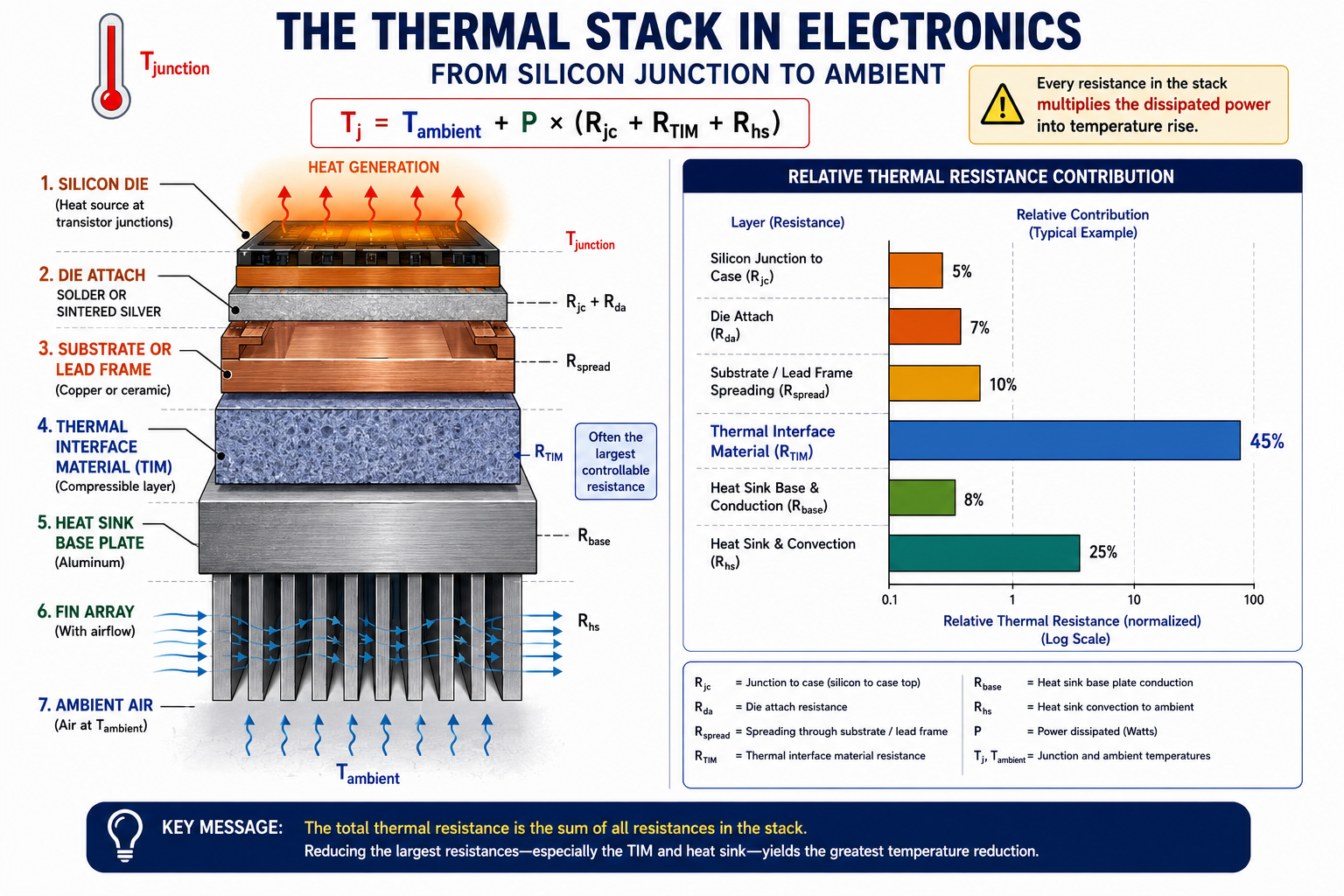
    The Thermal Stack in Electronics, From Silicon Junction to Ambient A vertical cross-section diagram showing the complete thermal resistance stack from silicon die to ambient air. From top to bottom: Silicon die (heat source, orange glow indicating heat generation at transistor junctions); Die attach solder or sintered silver (thin layer, labeled R_jc + R_da); Substrate or lead frame (copper or ceramic); Thermal interface material, TIM (compressible layer, labeled R_TIM with callout 'Often the largest controllable resistance'); Heat sink base plate (aluminium); Fin array with airflow arrows (labeled R_hs with airflow direction arrows); Ambient air (labeled T_ambient). On the right side, a vertical thermal resistance bar chart shows the relative contribution of each layer: TIM is the tallest bar (largest resistance), followed by heat sink, then die attach, then substrate, then spreading resistance. At the top, a thermometer icon labeled T_junction with the equation: T_j = T_ambient + P × (R_jc + R_TIM + R_hs). The message: every resistance in the stack multiplies the dissipated power into temperature rise.

    Thermal simulation allows engineers to predict temperature distributions in electronics assemblies before hardware is built, helping identify thermal risks, optimize cooling, and evaluate worst-case operating conditions.1

    The power of the framework is that it decomposes the thermal problem into individual resistances that can be independently analyzed, optimized, and validated. Each resistance element has a physical identity (die attach, TIM, heat sink), a formula or datasheet source for its value, and a set of design variables that control it. Simulation’s role is to compute these resistances accurately for the actual three-dimensional geometry, something the 1D formula cannot do for complex geometries, and to identify which resistance elements dominate the total, guiding optimization effort toward the highest-leverage design changes.

    Resistance ElementSymbolFormula / SourceTypical Value RangeWhat It GovernsHow to Reduce It
    Junction to case (die)R_jcProvided in component datasheet; governed by die size, bond wire layout, die attach material0.1–5.0 °C/W for ICs; 0.01–0.5 °C/W for power modulesMaximum power density the die can dissipate before junction temperature is exceededLarger die area; better die attach material (sintered silver vs solder); flip-chip vs wire bond
    Die attach (solder/adhesive)R_dat/(k × A); t = thickness, k = thermal conductivity, A = area0.05–0.5 °C/W; sintered silver ~0.01 °C/WHeat flow from die to substrate; first interface resistance below dieReduce solder thickness; use sintered silver (k=200 W/mK) vs SAC solder (k=57 W/mK); maximize die attach area
    Substrate / PCB spreadingR_spreadDepends on copper layer count, via density, board thickness0.5–5.0 °C/W for FR4 PCB; 0.1–1.0 °C/W for metal-core PCB (MCPCB)Lateral heat spreading from component footprint to board area available for convectionAdd copper pours; use thermal vias under component; switch to MCPCB or ceramic substrate for high-flux components
    Thermal interface material (TIM)R_TIMt/(k × A); k = 0.5–80 W/mK depending on TIM type0.05–1.0 °C/W; phase-change TIM ~0.1 °C/W; thermal paste ~0.2 °C/W; dry contact ~1.0 °C/WInterface between component case and heat sink, largest variable resistance in most systemsUse higher-k TIM; minimize bond line thickness (BLT); ensure surface flatness < 25 µm for paste/phase-change TIM
    Heat sink (fin + base)R_hs1/(h × A_fin); h = convection coeff, A_fin = fin area0.1–5.0 °C/W natural convection; 0.02–0.5 °C/W forced convectionConvection from heat sink to ambient air, governs total system thermal resistance floorIncrease fin area; reduce fin pitch for forced convection; use vapor chamber or heat pipe for spreading
    Case to ambient (no heat sink)R_caComplex, governed by board layout, enclosure, airflow2–20 °C/W for natural convection in enclosureTotal temperature rise from component case to ambient when no dedicated heat sink is usedAdd local copper thermal pad; ensure airflow path; space high-power components for mutual air convection
    PCB to ambient (conduction-cooled)R_boardDepends on copper layer count and conduction path to chassis1–10 °C/W from component to chassis edgeHeat flow via PCB copper to chassis ground plane, dominant path in conduction-cooled military/space electronicsMaximize copper fill between component and chassis attachment; use copper-core PCB; minimize PCB-to-chassis thermal resistance

    When the 1D Model Fails: The Spreading Resistance Problem

    The 1D thermal resistance model assumes heat flows in one direction, from the die straight down through the stack to the ambient. In reality, heat spreads laterally through every layer it passes through, expanding the effective heat transfer area as it moves away from the concentrated die heat source. This spreading increases the effective area for convection and reduces the thermal resistance below the 1D prediction, which sounds beneficial, but the spreading also creates lateral temperature gradients that the 1D model misses entirely

    Spreading resistance (Rspread) depends on the heat-source area, spreading-layer area, layer thickness, and thermal conductivity. For a small 5 × 5 mm die on a large 150 × 100 mm PCB, a simple 1D model can underestimate the local temperature because it does not capture how heat spreads outward from the die.

    A 2D or 3D thermal simulation captures this temperature gradient and shows whether the design is limited by poor heat spreading—requiring more copper or thermal vias—or by insufficient convection area, which may require a heat sink or increased airflow.

    Thermal simulation software such as SimScale enables engineers to model heat transfer, temperature distribution, and cooling performance before physical prototypes are built.

    The Effect of Adjacent Components: The Mutual Heating Problem

    In a densely populated PCB, every high-power component raises the local ambient temperature for its neighbors. A component that dissipates 3W in isolation might operate at 55°C junction temperature. The same component placed 10mm from a 5W DSP, which raises the local air temperature by 15°C through its convective plume, operates at 70°C. This mutual heating effect is invisible to single-component thermal analysis and is one of the most common causes of field failures in products where each individual component was analyzed in isolation and found to be thermally safe.

    System-level PCB thermal simulation, modeling the entire board with all components, their power dissipations, and the enclosure airflow, captures mutual heating automatically. The temperature at each component location includes contributions from all neighbors, not just the component’s own self-heating. The highest-risk components in a dense layout are not necessarily the highest-power ones, they are the ones with high thermal sensitivity (steep Arrhenius slope) placed in the thermal shadow of high-power neighbors. Identifying these components requires system-level simulation, not component-level analysis.

    Thermal Simulation Fidelity Levels: Choosing the Right Tool

    Electronics thermal simulation spans seven distinct fidelity levels, from a spreadsheet thermal resistance calculation to a full conjugate heat transfer CFD model with turbulent airflow, radiation, and thermal-structural coupling. Choosing the right fidelity level for each design decision is as important as building an accurate model, over-specifying the fidelity wastes time and compute resources on information that is not needed for the current design decision; under-specifying misses the physics that governs the outcome. The following table maps each method to its physics, accuracy, cost, and optimal use case.

    Tool / MethodPhysics CapturedAccuracy LevelComputational CostBest ForLimitation
    Thermal resistance network (1D/lumped)Conduction only; 1D steady-state from junction to ambient via Rth chainOrder-of-magnitude; ±20–50% for complex geometriesNegligible, spreadsheet calculationEarly design, budgeting junction temperature, comparing cooling strategies at system levelCannot predict spreading resistance, temperature gradients within PCB, or hotspot location
    2.5D PCB thermal analysis (layer-averaged)Conduction through PCB layers; simplified convection boundary; copper spreadingModerate, ±10–20% for temperature riseLow, seconds to minutesPCB layout thermal optimization; identifying hotspot components; copper pour placementMisses 3D effects; cannot model component-level airflow; simplified convection not accurate in ducted or complex enclosures
    3D conduction FEA (no CFD)Full 3D conduction; radiation (if included); boundary convection from convection coefficientsGood, ±5–15% with accurate convection coefficientsMedium, minutes to hours for detailed PCB modelComponent-level thermal analysis; heat spreader design; TIM optimization; conduction-cooled board designConvection coefficient is input, not computed, accuracy limited by quality of h values; cannot predict airflow-dependent cooling
    Conjugate heat transfer CFD (3D coupled)Full 3D conduction in solids + Navier-Stokes airflow; radiation optional; buoyancy for natural convectionHigh, ±3–10% for T_junction and flow patternsHigh, hours to days for full system modelEnclosure thermal design; heat sink optimization; natural convection systems; blower/fan performance in complex geometriesHigh mesh count for simultaneous fluid and solid domains; long run time limits parametric exploration speed
    Compact thermal model (JEDEC DELPHI)Behavioural model representing IC package as network of resistances calibrated to detailed modelGood, matches detailed model within 5–10% across board conditionsLow, component is a simplified resistance networkSystem-level analysis with many components; board-level thermal map without modeling every component in detailMust be calibrated from detailed model or datasheet; accuracy degrades outside calibration envelope
    Transient thermal analysis (FEA/CFD)Time-dependent conduction and convection; thermal mass (capacitance) of all elementsHigh for transient profiles; depends on material Cp accuracyHigh, many time steps at full 3D model costPower cycling life prediction; junction temperature during pulsed loads; thermal runaway analysis; Tj-vs-time under startupThermal capacitance data (Cp, density) must be accurate; long run times for slow thermal systems (battery packs, enclosures)
    Thermal-structural coupled (FEA)Conduction FEA feeding temperature field into structural FEA; thermal stresses and warpage computedStructural accuracy limited by thermal input accuracy; ±5–15% for stress if temperature is accurateHigh, two coupled analysesSolder joint fatigue prediction; PCB warpage; package CTE mismatch stress; connector retention under thermal cyclingRequires both accurate thermal model and accurate structural model; CTE mismatch data must be source-verified

    The Compact Thermal Model: Bridging Component and System Analysis

    The JEDEC DELPHI compact thermal model standard provides a practical solution to the tension between component-level accuracy and system-level analysis efficiency. A JEDEC DELPHI model represents a complete IC package as a behavioural network of thermal resistances calibrated to match the detailed package thermal simulation across a range of board conditions, different copper areas, airflow rates, and power levels. The compact model captures the package’s thermal behaviour correctly without requiring the analyst to model every internal layer of the package explicitly.

    The compact model’s input is the power dissipated by the component; its output is the junction temperature, given the board thermal conditions at the component’s attachment footprint. Because the model is computationally trivial (a small network of resistances), boards with 50 to 500 components can be analyzed in minutes using compact models for all components, a board-level analysis that would take days or weeks if every component were modeled in full 3D detail. The tradeoff: compact models are only accurate within their calibration envelope, and their accuracy degrades if the board conditions deviate significantly from the conditions under which they were calibrated.

    The CFD Conjugate Heat Transfer Model: When Full Physics Is Required

    Conjugate heat transfer (CHT) CFD simultaneously solves the Navier-Stokes equations for the fluid domain (airflow in the enclosure or heat sink) and the heat conduction equation for the solid domain (PCB, components, heat sink, enclosure), coupling them at all fluid-solid interfaces. The fluid temperature affects the solid temperature through convection; the solid temperature affects the fluid density and viscosity through buoyancy and property variation. CHT CFD is the only method that correctly computes the convection heat transfer coefficient h for complex enclosure geometries, the h that all lower-fidelity methods require as an input.

    The applications where CHT CFD is necessary rather than optional: natural convection systems (where buoyancy-driven flow depends on the temperature field in a coupled manner that cannot be prescribed as a boundary condition), complex forced convection with multiple airflow paths and obstructions, fan operating point determination in a specific duct geometry, and any system where the thermal design is being optimized rather than validated. A heat sink fin pitch optimization without CHT CFD is not an optimization, it is a guess, because the convection coefficient and pressure drop change with fin pitch in ways that cannot be captured by a simple h boundary condition applied to a conduction-only model.

    Thermally Activated Failure Mechanisms: What Simulation Must Predict

    The value of thermal simulation in electronics is not temperature for its own sake, it is failure rate prediction. Every thermally activated failure mechanism has a quantitative relationship between temperature and failure rate, described by the Arrhenius equation: failure rate scales as exp(-E_a / kT), where E_a is the activation energy, k is Boltzmann’s constant, and T is the absolute temperature in Kelvin. The implication is direct: every 10°C reduction in junction temperature approximately halves the failure rate for mechanisms with activation energy around 0.7 eV, the most common range for semiconductor failure mechanisms. Conversely, every 10°C increase approximately doubles the failure rate.
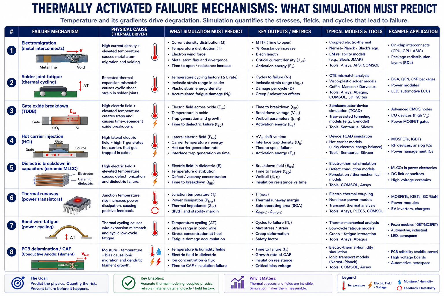
    Thermally Activated failure mechanisms

    The failure rate relationship means that the thermal simulation’s accuracy requirement is set by the failure rate sensitivity, not by an absolute temperature accuracy. For a mechanism with 2x failure rate per 10°C, a 10°C error in junction temperature prediction doubles or halves the predicted failure rate, producing a reliability prediction that is off by a factor of 2 from the actual field failure rate. For safety-critical electronics (automotive, aerospace, medical) where the reliability target may be 1,000 to 10,000 FIT (failures per billion device hours), a factor-of-2 reliability prediction error is the difference between a compliant design and a field recall.

    Failure MechanismTemperature DependenceSimulation Output NeededArrhenius Acceleration Factor (per 10°C)Design Target
    Electromigration (metal interconnects)Exponential, activation energy 0.7–1.0 eV; doubles failure rate every 8–12°CPeak metal layer temperature; current density distribution at via and metal necks2.0–2.8x per 10°C at operating rangeKeep Tj < 85°C for standard ICs; < 105°C for automotive; via current density < 5×10^5 A/cm^2
    Solder joint fatigue (thermal cycling)Coffin-Manson: N_f proportional to delta_T^{-alpha}; cycles to failure drop with temperature rangeTemperature range delta_T per cycle; mean temperature Tm; plastic strain amplitude in solderCycle life halves for every 15–20°C increase in delta_TMinimize delta_T per cycle; keep Tj < 100°C for SnAgCu solder on FR4; use underfill for fine-pitch BGA
    Gate oxide breakdown (TDDB)Strong temperature dependence, activation energy 0.7–1.1 eV; time-to-breakdown halves every 7–10°C above thresholdGate oxide temperature, closely tracks junction temperature2.0–3.0x per 10°CKeep Tj < datasheet maximum; typically 125°C for silicon CMOS; 150–175°C for automotive-grade
    Hot carrier injection (HCI)Worst at intermediate temperatures (25–75°C); less dominant at highest temperatures vs electromigrationPeak channel electric field; device current density; junction temperature~1.5–2.0x per 10°C for drain current stress | weakly temperature-dependentVoltage derating at elevated temperature; transistor sizing to limit peak field
    Dielectric breakdown in capacitors (ceramic MLCC)Exponential, time to failure scales as exp(-E_a/kT); strong dependence above rated temperatureCapacitor body temperature; voltage stress2–4x per 10°C above rated temperatureDerate voltage to 50–80% of rated at operating temperature; keep temperature < 85°C or use 125°C rated parts
    Thermal runaway (power transistors)Positive feedback: higher T → lower R_ds(on) for BJT → more current → higher TDynamic junction temperature during switching; thermal impedance Z_th transientRunaway threshold: depends on device and load line intersectionEnsure load line does not cross device’s safe operating area (SOA); use thermal protection circuit; verify Z_th(t) under pulse conditions
    Bond wire fatigue (power cycling)Thermal cycling between bond wire and die: CTE mismatch drives plastic deformation at heel of bondNumber of power cycles; peak and trough Tj per cycle; bond wire temperature gradientCycle life halves for every 10–15°C increase in delta_Tj per power cycleLimit power cycle amplitude; use heavy aluminium or copper wire for power modules; use silver sintering instead of wire bond where possible
    PCB delamination / CAF (Conductive Anodic Filament)Accelerated by high temperature + high humidity; CAF growth rate exponential with temperaturePCB temperature map; identify copper features at risk of CAF between adjacent conductors3–5x per 10°C acceleration in highly accelerated life test (HALT/HAST)Limit PCB temperature < 85°C for standard FR4; use halogen-free low-CTE laminates for high-reliability applications

    Electromigration: The Temperature-Current Density Interaction

    Electromigration, the migration of metal atoms along grain boundaries under the force of electron momentum transfer, is the dominant long-term failure mechanism in semiconductor interconnects. The Black’s equation for electromigration mean time to failure is: MTF = A × J^{-n} × exp(E_a / kT), where J is the current density in the metal conductor, n is typically 1–2 for modern interconnects, and E_a is the activation energy (0.7–1.0 eV depending on the metal and interface).

    Thermal simulation for electromigration must provide two outputs: the temperature at each metal layer (to evaluate the exp(E_a/kT) term) and the current density distribution (for the J^{-n} term). In practice, current density is computed by electrical simulation (IR drop analysis), and temperature is computed by thermal simulation with the current-density-dependent Joule heating as the heat source. The two simulations are coupled: current density generates heat, heat changes resistivity, changed resistivity changes current distribution. For high-current-density designs, an electrothermal co-simulation that couples the electrical and thermal solvers is required to correctly capture this interaction, a thermal-only simulation with fixed current density underestimates the temperature at high-current vias and metal necks.

    Solder Joint Fatigue: Linking Thermal Cycling to Mechanical Failure

    Solder joint fatigue is the most common thermally driven mechanical failure mode in electronic assemblies. The failure mechanism is thermal cycling: as the PCB temperature rises during operation and falls during standby, the differential thermal expansion between the component package (CTE ~6–15 ppm/°C depending on package type) and the PCB (CTE ~14–18 ppm/°C for FR4) drives plastic deformation in the solder joint. Each thermal cycle accumulates a small increment of plastic strain; after enough cycles, the accumulated damage initiates a fatigue crack that propagates to electrical open failure.

    The Coffin-Manson relationship for solder fatigue is: N_f = C × (delta_epsilon_p)^{-alpha}, where N_f is the cycles to failure, delta_epsilon_p is the plastic strain range per cycle, and C and alpha are material constants (alpha ≈ 1.9 for SnAgCu lead-free solder). Thermal simulation provides the temperature range delta_T at the solder joint level; structural simulation converts this temperature range to plastic strain amplitude using CTE mismatch, package geometry, and solder constitutive behavior. Neither the thermal model alone nor the structural model alone can predict solder fatigue life, the coupled thermal-structural analysis is required, and accuracy demands that both the temperature field and the material plasticity model be correctly specified.

    Heat Sink Design Optimization Through Simulation

    Heat sink design is one of the most valuable applications of thermal simulation because the relationship between fin geometry and thermal performance is highly nonlinear. Simple analytical correlations can estimate the performance of an isolated fin array under uniform airflow, but they cannot fully capture real-world effects such as flow non-uniformity between fins, pressure drop and its impact on fan performance, heat spreading through the base, or thermal contact resistance at the component interface.
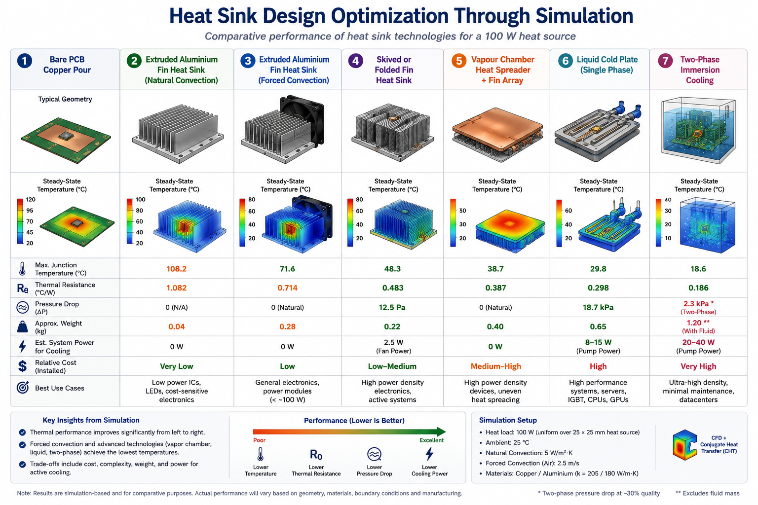
    Heat sink design optimization through simulation

    Conjugate heat transfer (CHT) CFD captures these effects together, allowing engineers to optimize the heat sink rather than simply select a standard catalog design. Fin pitch, height, thickness, and base thickness can be varied systematically to identify the geometry that provides the lowest thermal resistance for a specific fan, enclosure, power density, and airflow constraint.

    Heat Sink TypeThermal Resistance RangeAirflow RequirementPower Density (W/cm²)Typical ApplicationKey Design Variable for Simulation
    Bare PCB copper pour10–30 °C/W component-to-ambientNone (natural convection from copper surface)< 0.1 W/cm²Low-power ICs, microcontrollers, small regulators on consumer PCBCopper pour size and shape; distance to board edge; copper layer count
    Extruded aluminium fin heat sink (natural convection)2–10 °C/WNone, buoyancy-driven natural convection between fins0.1–0.5 W/cm²Linear voltage regulators, small power supplies, industrial control modulesFin height, pitch, thickness, base plate thickness, optimised by CFD natural convection sweep
    Extruded aluminium fin heat sink (forced convection)0.2–2.0 °C/W0.5–5 m/s air velocity across fins0.5–5 W/cm²Server CPUs, power amplifiers, motor drives, industrial electronicsFin pitch optimisation for given fan curve; pressure drop vs flow rate; fan operating point intersection
    Skived or folded fin heat sink0.05–0.5 °C/W forced convection2–10 m/s; dedicated blower or axial fan2–20 W/cm²High-performance CPUs/GPUs, IGBT power modules, telecom base stationsVery thin fin pitch (0.5–1.5 mm) requires CFD for accurate pressure drop; fin-to-fin airflow uniformity
    Vapour chamber heat spreader + fin array0.02–0.2 °C/W (spreading resistance near zero)Any, separate from spreading function10–100 W/cm² on die; spreads to fin areaHigh-flux processors (>100W TDP), GPU packages, 5G mmWave power amplifiersEffective spreading resistance vs die size; interface resistance at vapour chamber base; fin array optimisation above VC
    Liquid cold plate (single phase)0.01–0.2 °C/W liquid-to-coolantCoolant flow rate 1–10 L/min at 20–60°C inlet50–500 W/cm²High-power server CPUs, IGBT stacks in EV inverters, data centre liquid coolingInternal channel geometry (serpentine, pin-fin, micro-channel); pressure drop vs flow; coolant inlet/outlet temperature
    Two-phase immersion cooling0.001–0.05 °C/W effectivePassive (pool boiling) or pumped two-phase> 500 W/cm² peak; > 100 W/cm² sustainableExtreme density data centres, HPC accelerator nodes, power electronics in electrified aviationBoiling curve (heat flux vs superheat); nucleation site density; vapour bubble dynamics, requires specialised two-phase CFD

    Fin Pitch Optimization: Where CFD is Essential

    The fin pitch optimization problem illustrates why CFD cannot be replaced by analytical formulas for heat sink design. Decreasing fin pitch increases the fin area per unit volume (good for heat transfer) but also increases the flow resistance through the fin channels (bad, reduces airflow for a given fan pressure). The optimal fin pitch is the one that maximizes heat transfer given the actual fan operating point, which itself depends on the fin array pressure drop.

    The analytical approach: compute heat transfer coefficient h for a given pitch using the Dittus-Boelter correlation for turbulent channel flow; compute fin efficiency; compute thermal resistance. This approach misses: the entrance length effect (h is higher near the leading edge of each fin); the fin tip-to-shroud clearance effect (bypass flow reduces effective airflow through fins); the heat sink inlet flow non-uniformity; and the fan curve intersection with the system resistance curve. Each of these effects changes the optimum pitch by 10 to 30 percent.

    CFD optimization workflow: parametrically vary fin pitch from 1.0mm to 4.0mm in 0.5mm steps, holding fin height, base thickness, and fan constant. For each pitch, the CHT CFD simulation computes: the actual airflow rate through the fin array (from the fan curve intersection with the computed system resistance), the local heat transfer coefficient distribution along each fin, the fin temperature distribution, and the junction temperature. The pitch that minimizes T_junction is the optimal design, and the result is typically 15 to 30 percent better thermally than the pitch selected by the analytical approach alone.

    Vapour Chamber Integration: Simulation for Spreading-Limited Systems

    When the die heat flux exceeds approximately 50 W/cm², the spreading resistance in a solid aluminium or copper heat sink base becomes the dominant thermal resistance, the fin array performance is irrelevant if the heat cannot spread from the die to the fin area fast enough. Vapour chambers, flat two-phase heat spreaders that use the evaporation-condensation cycle of a working fluid (typically water) to transport heat laterally with near-zero effective thermal resistance, address this limitation.

    Thermal simulation of vapour chamber systems replaces the high spreading resistance of a conventional solid base with the much higher effective thermal conductivity of the vapour chamber. This effective conductivity is typically modeled at 5,000–50,000 W/mK, compared with about 200 W/mK for copper and 150 W/mK for aluminium.

    The simulation applies this equivalent conductivity to the spreading layer, with conduction FEA or conjugate heat transfer (CHT) CFD used above and below it. The result is a more uniform base temperature and smaller temperature gradients across the heat sink. This also improves fin efficiency because the fins operate at more similar temperatures instead of the fins directly above the die running significantly hotter than those farther away.

    Power Cycling and Transient Thermal Analysis

    Steady-state thermal analysis answers the question: what is the junction temperature when the device has been operating at constant power long enough for the temperature to stabilize? Transient thermal analysis answers the question: what is the junction temperature at every moment in time during a time-varying power profile? For many electronics applications, the transient answer is more important than the steady-state answer, peak junction temperature may occur during a brief power spike that lasts milliseconds, not during sustained operation, and the failure mechanisms that respond to peak temperature (gate oxide breakdown, hot carrier injection, thermal runaway) are determined by the transient peak, not the steady-state average.

    The Thermal Impedance Z_th: The Transient Thermal Resistance

    The transient thermal behaviour of an electronic component is described by its thermal impedance Z_th(t), the ratio of junction temperature rise to applied power, as a function of time after a power step is applied. Unlike the steady-state thermal resistance R_th, which is a single number, Z_th(t) is a function that starts near zero (immediately after the power step, only the small thermal mass of the die itself has been heated) and rises asymptotically to R_th as the heat diffuses through all the thermal layers to the ambient.

    The Z_th(t) curve is directly measurable from the die junction using the electrical test method (JEDEC JESD51-14) and is provided in power semiconductor datasheets as a standard parameter. For FEA thermal simulation, Z_th(t) is a primary validation target: a correctly built transient thermal model should match the measured Z_th(t) curve within 5 to 10 percent across the entire time range from 1 microsecond to steady state. Discrepancies at short time scales indicate incorrect material heat capacity (Cp × rho × volume) for the die or die attach; discrepancies at long time scales indicate incorrect thermal resistance in the package-to-board or board-to-ambient path.

    Power Cycling Reliability: Simulation for Automotive and Industrial Applications

    Power cycling, the repeated thermal cycling of a power semiconductor under electrical load, with junction temperature swings of 50 to 150°C per cycle, is the most accelerated degradation mechanism in power electronics. IGBTs in electric vehicle inverters may experience millions of power cycles over the vehicle lifetime, driven by the motor control current profile that generates hundreds of milliseconds-long current pulses at each motor commutation. Each current pulse heats the IGBT junction; each pulse off-time cools it. The repeated thermal strain accumulates fatigue damage in the bond wires and the solder die attach layers until one of them fails.

    Transient thermal simulation for power cycling reliability requires: the junction temperature waveform T_j(t) for the actual drive cycle (current profile, ambient temperature, cooling conditions); the extraction of delta_T_j (the peak-to-trough junction temperature swing per power cycle); the mean junction temperature T_j_mean; and the number of cycles per hour of operation. These are fed into the power cycling lifetime model (typically a modified LESIT model or the Coffin-Manson-Arrhenius model from IEC 60747): N_f = A × (delta_T_j)^{-alpha} × exp(E_a / k T_j_mean). The simulation output directly predicts the number of power cycles to failure, which maps to vehicle lifetime in hours of operation given the drive cycle statistics.

    Worked Example: Power Cycling Lifetime Calculation for EV Inverter IGBT
    GIVEN:
      IGBT module: 650V, 400A, R_jc = 0.04 °C/W, P_sw = 800W peak (switching losses)
      Drive cycle: 200ms ON (800W) / 200ms OFF, 2.5 Hz cycling frequency
      Cooling: liquid cold plate, T_coolant_in = 65°C, R_thermal_cold_plate = 0.015 °C/W
      Z_th(t) for 200ms pulse: Z_th(0.2s) = 0.028 °C/W (from datasheet curve)

    STEP 1: Junction temperature during ON pulse
      T_j_peak = T_coolant + P × [R_cold_plate + Z_th(0.2s)]
               = 65 + 800 × [0.015 + 0.028]
               = 65 + 800 × 0.043
               = 65 + 34.4
               = 99.4 °C

    STEP 2: Junction temperature at end of OFF pulse
      After 200ms OFF, junction cools toward steady-state T_j at zero power.
      T_j_min ≈ T_coolant + P_idle × R_total ≈ 65 + 10 × 0.055 ≈ 65.6 °C
      (P_idle = 10W conduction losses at zero switching)

    STEP 3: Power cycling parameters
      delta_T_j = T_j_peak - T_j_min = 99.4 - 65.6 = 33.8 °C
      T_j_mean  = (99.4 + 65.6) / 2 = 82.5 °C = 355.5 K

    STEP 4: Lifetime prediction (modified LESIT model)
      N_f = 302,500 × (delta_T_j)^{-5.039} × exp(7823 / T_j_mean)
          = 302,500 × (33.8)^{-5.039} × exp(7823 / 355.5)
          = 302,500 × 1.73e-8 × exp(22.01)
          = 302,500 × 1.73e-8 × 3.61e9
          = 18,900,000 cycles

    STEP 5: Vehicle lifetime
      At 2.5 Hz cycling: cycles/hour = 2.5 × 3600 = 9,000 cycles/hr
      Hours to failure: 18,900,000 / 9,000 = 2,100 hours
      At 15,000 km/year, 100 km/hr average: 150 hours/year drive time
      Vehicle lifetime: 2,100 / 150 = 14 years, MEETS 10-year target

    SENSITIVITY: If T_coolant rises to 75°C (hot summer, stuck traffic):
      T_j_peak = 109.4°C, delta_T_j = 43.8°C
      N_f drops to ~4,800,000 cycles → 533 hours → 3.6 years, FAILS
      ACTION: Either improve cold plate or limit switching losses at high

    Thermal-Structural Coupling: PCB Warpage and Solder Joint Stress

    Thermal-structural coupling, using the temperature field from a thermal simulation as the input load to a structural FEA model, extends thermal simulation from temperature prediction to mechanical failure prediction. The two most important thermal-structural applications in electronics design are PCB warpage during reflow soldering (which determines whether components can be placed and soldered reliably) and solder joint fatigue under thermal cycling in service (which determines the product’s long-term reliability in the field).

    PCB Warpage During Reflow: The Assembly Yield Problem

    During reflow soldering, lead-free SAC assemblies typically reach peak temperatures of 230–260°C before cooling. Differences in thermal expansion between the PCB, components, and solder, combined with laminate relaxation at high temperatures, can cause permanent board warpage after cooling. Excessive warpage can lead to solder bridging, solder voiding, and head-in-pillow defects, particularly in large BGA packages.

    Thermal-structural simulation of reflow warpage accounts for temperature-dependent material behavior, CTE mismatch between PCB layers and components, and the complete reflow temperature profile. The analysis predicts warpage throughout the heating and cooling cycle and after the board returns to room temperature. Engineers can then adjust the PCB stackup, copper distribution, or stiffening features before production, reducing assembly defects and improving manufacturing yield.

    Solder Joint Stress Under Thermal Cycling: Field Life Prediction

    For products that will experience thermal cycling in service, automotive electronics between -40°C and 125°C, outdoor telecom equipment between -40°C and 85°C, consumer electronics in daily use between 15°C and 85°C, solder joint fatigue life prediction through thermal-structural simulation is the primary reliability design tool. The simulation provides what no accelerated test can provide: a physics-based prediction of solder joint life at the actual field thermal cycle profile, mapped to an equivalent number of field cycles from the accelerated test conditions.

    The thermal-structural workflow for solder joint reliability involves four steps: (1) simulate the thermal cycle to determine the temperature history at each solder joint; (2) use temperature-dependent SAC solder properties to calculate plastic strain accumulation during each cycle; (3) apply a Coffin-Manson fatigue model to estimate cycles to failure; and (4) compare the predicted fatigue life with the expected number of thermal cycles over the product’s design life.

    The most critical solder joints are typically located at the corners of large BGA, QFP, and LGA packages. These joints have the greatest distance from the package center, known as the distance to neutral point (DNP). Because CTE mismatch displacement increases with DNP, corner joints generally experience the highest cyclic strain and fatigue risk.

    Battery and EV Power Electronics: The Emerging Frontier

    The electrification of transportation has created two new high-priority applications for thermal simulation in electronics: battery pack thermal management and high-voltage power electronics cooling for inverters, DC-DC converters, and on-board chargers. Both applications involve higher power densities, higher voltages, and more demanding duty cycles than traditional electronics, and both have failure modes (thermal runaway in batteries, bond wire fatigue in inverter IGBTs) where thermal simulation directly prevents catastrophic failures.

    Battery Pack Thermal Simulation: Preventing Thermal Runaway

    Thermal runaway, the uncontrolled self-heating of a lithium-ion battery cell that leads to electrolyte vaporization, separator failure, and potentially fire, is the catastrophic failure mode that battery thermal management simulation is specifically designed to prevent. The simulation challenge is that thermal runaway is a nonlinear positive feedback event: heat generation from the electrochemical reactions in the cell increases exponentially with temperature, and if the heat generation exceeds the heat removal capacity of the thermal management system, the temperature rises until the cell vents and ignites.

    Battery thermal simulation supports thermal runaway prevention through three key analysis types: steady-state thermal analysis for normal operation, transient thermal analysis for fast charging and peak discharge, and thermal propagation analysis for single-cell runaway scenarios. These analyses help verify cell temperatures, predict temperature rise during high-power operation, and determine how effectively the thermal management system limits heat propagation to neighboring cells.

    Thermal propagation analysis is particularly important for EV battery safety, where regulations such as UN ECE R100 and GB/T 38661 address thermal safety and propagation risks. Simulation helps engineers evaluate these scenarios early, identify thermal management weaknesses, and improve battery pack safety before physical testing.

    SiC and GaN Power Electronics: Higher Temperature, Higher Frequency

    Silicon carbide (SiC) and gallium nitride (GaN) power semiconductors are increasingly replacing silicon IGBTs in high-efficiency power electronics. Their ability to switch at higher frequencies with lower switching losses enables smaller passive components and higher power density. However, their higher power density also creates new thermal-management challenges. SiC MOSFETs can operate at junction temperatures up to 175°C, while some GaN devices can reach 200°C, creating high local heat fluxes in compact packages.

    Thermal simulation for SiC and GaN systems must account for temperature-dependent material properties across a wider temperature range than traditional silicon-based designs. The power loop’s parasitic inductance also affects switching speed and losses, creating stronger coupling between electrical and thermal behavior. For high-fidelity analysis, electrothermal co-simulation simultaneously solves the circuit and thermal equations, capturing how switching losses affect temperature and how temperature, in turn, changes device performance.

    The Electronics Thermal Simulation Workflow: From Schematic to Reliability Prediction

    The complete thermal simulation workflow in electronics design follows a defined sequence of increasing fidelity, with decision gates at each stage that determine whether to proceed, iterate, or escalate to a higher-fidelity model. This workflow maps directly to the design stage, the fidelity of the thermal analysis should match the maturity of the design, with simple models at early concept stages and full CHT CFD and thermal-structural analysis at the detailed design stage before manufacturing release.

    1. Schematic / concept stage, 1D thermal resistance network: Compute T_junction for each high-power component using the datasheet R_jc, estimated board R_ca, and the cooling system R_hs. Identify components within 20°C of their maximum rated junction temperature. Flag these for closer attention in subsequent stages. This analysis takes hours and can be done in a spreadsheet before any PCB layout exists.
    2. PCB layout stage, 2.5D board-level thermal map: Import the PCB layout and component power dissipations. Run a 2.5D thermal analysis to generate the board temperature map. Identify hotspot locations and the components in the thermal shadow of high-power neighbors. Optimize copper pour placement, component spacing, and thermal via pattern based on the temperature map. This iteration loop runs in minutes per variant and can be completed within the PCB layout process.
    3. Detailed design stage, 3D conjugate heat transfer CFD: Build the full 3D enclosure model with fan or blower, PCB with all significant components, and detailed heat sink geometry. Run CHT CFD to determine the actual airflow distribution, the fan operating point in the system, the temperature distribution throughout the enclosure, and the junction temperatures of all critical components. Use this model to finalize heat sink geometry, fan selection, and component placement before tooling release.
    4. Reliability verification, thermal-structural coupled analysis: For the finalized design, run the coupled thermal-structural analysis to predict solder joint fatigue life under the field thermal cycle profile. Run transient analysis with the power profile to predict Z_th(t) correlation and peak junction temperature under pulsed loads. Verify that the design meets all thermal reliability targets before first article prototype builds.
    5. Prototype correlation, simulation update: Instrument the prototype with thermocouples or infrared measurement at key locations. Compare measured temperatures against simulation predictions. Update the simulation model to match measurements, typically by adjusting TIM thermal resistance and convection coefficients. The updated model becomes the validated model for design variant analysis and for extrapolating to environmental conditions not tested in the prototype phase.
    CRITICAL: Thermal Simulation Must Use Worst-Case Conditions, Not Typical
    One of the most common mistakes in electronics thermal simulation is analyzing only nominal conditions, typical power, 25°C ambient temperature, sea-level pressure, and unrestricted airflow. A design that passes under these conditions may still fail in the field when maximum power, high ambient temperature, altitude, and restricted airflow occur together.
    For reliable thermal design, simulations should evaluate worst-case operating conditions, including maximum power, maximum ambient temperature, reduced air density at altitude, and potential airflow restrictions such as clogged filters or blocked intakes. Nominal-condition analysis is useful for understanding normal operation, but worst-case thermal analysis is essential for establishing thermal compliance and reliability.

    Frequently Asked Questions

    Q: What is junction temperature and why is it the primary output of electronics thermal simulation?

    Junction temperature (Tj) is the temperature at the active semiconductor junction where switching and current conduction occur. It is the key output of electronics thermal simulation because semiconductor reliability models and datasheet temperature limits are based on Tj.

    Case or package temperature is lower than Tj because heat flows through the junction-to-case thermal resistance. For example, a device with a 60°C case temperature can still have a 125°C junction temperature if power dissipation creates a 65°C temperature difference. Accurate Tj prediction therefore requires thermal simulation or direct thermal measurement.

    Q: How accurate does thermal simulation need to be for electronics reliability prediction?

    The required thermal simulation accuracy depends on the failure mechanism and how close the device operates to its junction-temperature limit. For electromigration and other Arrhenius-based mechanisms, a ±5°C error can produce about a 1.4× error in failure-rate prediction, while a ±10°C error can produce roughly a 2× error, which may be unacceptable for safety-critical applications.

    For solder joint fatigue, accuracy in the temperature range (ΔT) per cycle is more important. A ±5°C error in ΔT can change predicted fatigue life by approximately 25%. In practice, validated CHT CFD models can achieve ±3–8°C junction-temperature accuracy compared with thermocouple measurements. However, uncertainty in input power and ambient-temperature distribution can often have a greater impact than simulation accuracy itself.

    Q: What is a thermal via and how does simulation determine how many are needed?

    A thermal via is a plated through-hole designed to transfer heat from a component’s top copper layer through the low-conductivity FR4 laminate to inner or bottom copper layers. PCB thermal simulation can optimize the via count and pattern by evaluating spreading resistance based on via diameter, spacing, fill material, and geometry.

    For example, a 4×4 array of 0.3 mm solder-filled vias at 0.6 mm pitch under a QFN package can reduce PCB spreading resistance by 40–60% compared with no thermal vias. For a 2 W device on standard FR4, this can reduce junction temperature by approximately 8–15°C.

    Q: What is the difference between thermal resistance and thermal impedance?

    Thermal resistance (Rth) is a steady-state measure of temperature rise per unit of power dissipation once the system reaches thermal equilibrium. Thermal impedance (Zth) is a transient measure that describes how temperature rises after a power step is applied. Zth starts near zero and gradually approaches Rth as heat spreads through the device and surrounding materials.

    This distinction is important for pulsed-power applications. For example, a device with an Rjc of 1.0°C/W may have a Zth of only 0.05°C/W at 1 ms, allowing much higher short-duration power without exceeding the maximum junction temperature. Thermal simulation should therefore account for both steady-state thermal resistance and transient thermal impedance.

    Q: Can I use a thermal simulation to replace thermal testing of prototypes?

    Thermal simulation should complement prototype testing, not replace it. Its purpose is to identify and resolve most thermal problems before the first prototype is built, turning prototype testing into a validation exercise rather than a problem-discovery exercise.

    Once the simulation is correlated with thermocouple or infrared measurements, the validated model can be used to evaluate design variants, operating conditions, and environmental scenarios that were not physically tested. The ideal workflow is simulate → prototype → validate → optimize. Simulation reduces interim test iterations, while physical testing remains essential for final qualification where required by standards such as AEC-Q and MIL-STD-810.

    Q: What material properties are most critical for accurate electronics thermal simulation?

    The material properties with the greatest impact on thermal simulation accuracy are:

    1. TIM thermal conductivity (kTIM): The thermal interface material between the component and heat sink can be a major source of thermal resistance. Its conductivity ranges from about 0.5–80 W/m·K, depending on the material.
    2. PCB through-plane conductivity (kz): FR4 typically has a low kz of about 0.3 W/m·K. Copper via fill can significantly improve heat transfer to inner layers, so the correct effective conductivity is important.
    3. Die-attach conductivity: Standard SAC solder has a conductivity of about 57 W/m·K, while sintered silver can reach approximately 200 W/m·K. Using incorrect values can distort the predicted thermal resistance below the die.
    4. Heat capacity (Cp × ρ): This is critical for transient analysis because it determines the thermal time constant and affects the predicted thermal impedance Zth(t).

    For reliable results, use material properties from supplier datasheets or certified databases rather than generic textbook values.

    Conclusion:

    The thermal failure mechanisms that govern electronics reliability, including electromigration, solder joint fatigue, gate oxide breakdown, and bond wire failure, are highly sensitive to temperature. Even a small error in junction temperature can significantly affect predicted failure rates. For products with demanding reliability targets, accurate thermal prediction is therefore a critical part of the design process.

    Thermal simulation provides engineers with a way to predict junction temperatures before prototypes exist and across a wide range of operating conditions. While a 1D thermal resistance model is useful for early estimates, it may miss mutual heating between components, PCB temperature gradients, airflow variations, and transient temperature peaks. These effects can shift junction temperature enough to produce non-conservative reliability predictions.

    The seven thermal simulation fidelity levels discussed in this article provide a practical path from early design screening to detailed validation. Simple thermal resistance models are useful for initial decisions, while CHT CFD, transient thermal analysis, and thermal-structural simulation provide greater detail when the design requires it. Used progressively and validated against physical testing, thermal simulation helps engineers identify thermal risks earlier, reduce prototype iterations, and build greater confidence in electronics reliability before production.

    Deepen your simulation knowledge with our guides on CFD vs wind tunnel testing, why simulation fails, FEA preprocessing, static vs dynamic analysis, and how leading industries deploy simulation to prevent failures and reduce development cost.
    1. IEEE Technology Navigator, “Thermal Management of Electronics,” IEEE. ↩︎
  • Why Simulation Fails Even With Good CAD Models (And How to Fix It)

    Why Simulation Fails Even With Good CAD Models (And How to Fix It)

    The geometry was perfect. It had been built by an experienced CAD designer who understood the manufacturing process, modeled every fillet to the correct radius, and exported a clean, watertight solid body that meshed without errors. The mesh quality metrics were excellent, Jacobian above 0.85, aspect ratio below 4:1 throughout, convergence confirmed with three mesh refinements. The boundary conditions matched the physical test setup. The material properties were from the certified material datasheet. Every box on the preprocessing checklist was checked.

    The simulation predicted a maximum stress of 187 MPa at the shaft shoulder. The shaft yielded at 220 MPa. The safety factor appeared to be 1.18, adequate for a non-critical application. The shaft failed in fatigue after 80,000 cycles. The laboratory fatigue test, run afterward to investigate the failure, showed a fatigue life of 85,000 cycles, consistent with the physical failure. The simulation had predicted 187 MPa of peak von Mises stress.

    The fatigue analysis used that number. What neither the simulation setup nor the fatigue analysis had accounted for was that the correct fatigue-driving stress was the signed maximum principal stress amplitude, and under the combined bending and torsion loading, the maximum principal stress amplitude was 312 MPa, not 187 MPa. The safety factor was not 1.18. It was 0.71.

    The failure was not caused by bad CAD. It was not caused by a mesh problem. It was not caused by wrong boundary conditions or incorrect material properties. It was caused by misidentifying which stress quantity drives fatigue failure, a postprocessing interpretation error that is entirely independent of the quality of the CAD model, the mesh, or any other preprocessing decision. This is the central reality of simulation accuracy: the overwhelming majority of simulation failures occur in the decisions the analyst makes about physics, modeling approach, and results interpretation, not in the geometric representation of the part.

    This article catalogs the twelve categories of simulation failure beyond geometry quality, provides the complete physics assumption error table for structural FEA, the eight most common postprocessing interpretation mistakes and how to avoid them, and the validation methods that catch errors before they propagate to wrong design decisions. The goal is a framework for understanding why simulation fails when the CAD model is not the problem, which is most of the time.

    The Complete Taxonomy of Simulation Failure

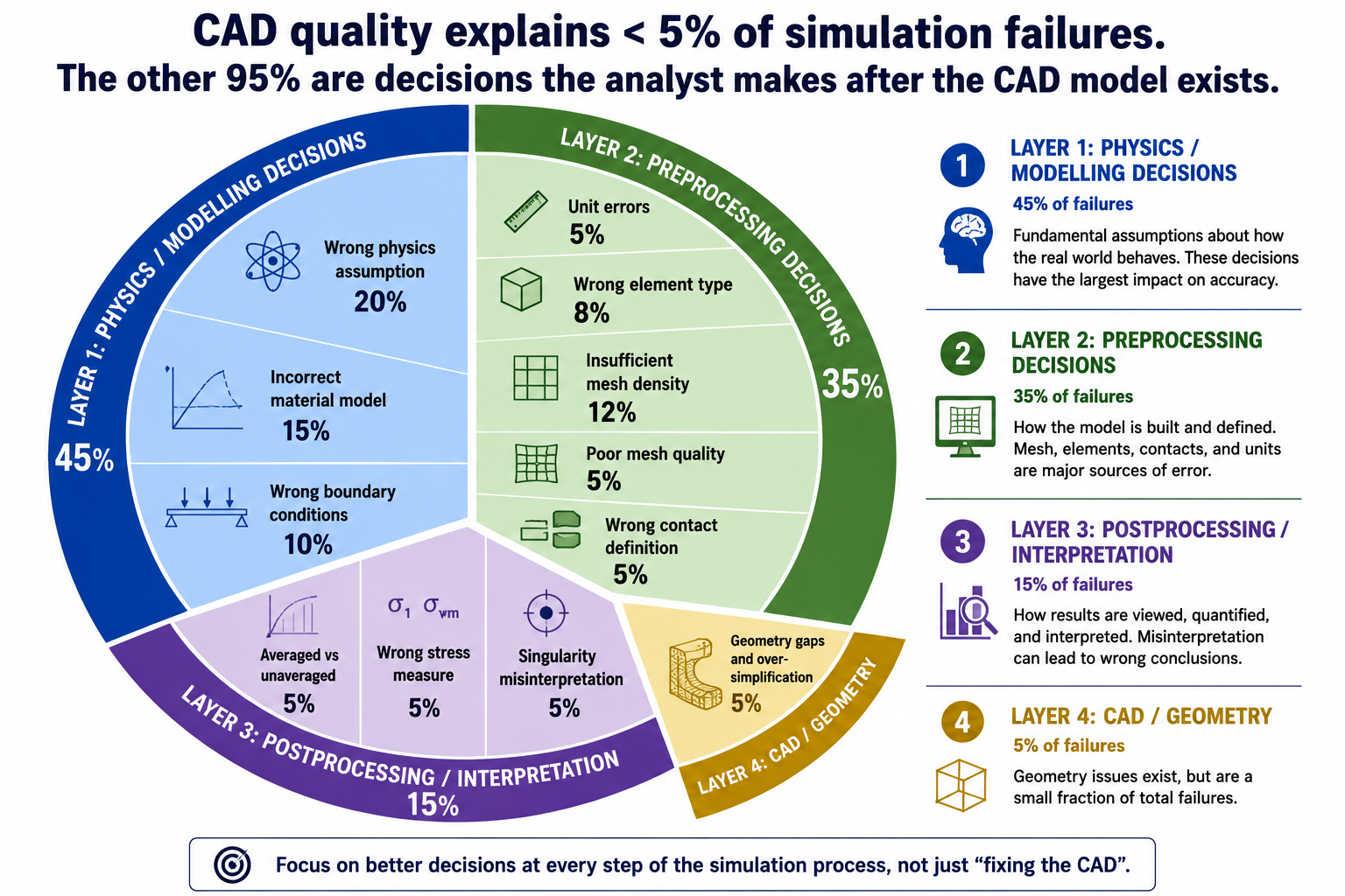
    Simulation failure, producing a result that does not represent the physical behavior of the structure, occurs at four distinct layers: physics and modelling decisions, preprocessing decisions, solver numerics, and postprocessing and interpretation. CAD geometry quality is a subset of preprocessing decisions and, when it is the problem, it typically manifests as mesh generation failure (which is obvious) or poor mesh quality (which is caught by quality metrics). The subtle failures, the ones that produce plausible-looking wrong results, occur almost entirely in physics assumptions and postprocessing interpretation, two layers that are completely independent of CAD quality.

    The FEA Error Taxonomy, Where Failures Actually Come From
ALT: A pie chart or treemap showing the distribution of FEA error sources across four layers. Layer 1 (Physics/Modelling Decisions) takes up approximately 45% of the area: subdivided into wrong physics assumption (20%), incorrect material model (15%), wrong boundary conditions (10%). Layer 2 (Preprocessing Decisions) takes up approximately 35%: subdivided into unit errors (5%), wrong element type (8%), insufficient mesh density (12%), poor mesh quality (5%), wrong contact definition (5%). Layer 3 (Postprocessing/Interpretation) takes up approximately 15%: subdivided into averaged vs unaveraged (5%), wrong stress measure (5%), singularity misinterpretation (5%). Layer 4 (CAD/Geometry) takes up approximately 5%: geometry gaps and over-simplification. The CAD layer is deliberately shown as the smallest segment to reinforce the article's thesis, geometry problems are a small fraction of total simulation failures. A bold label over the chart reads: 'CAD quality explains < 5% of simulation failures. The other 95% are decisions the analyst makes after the CAD model exists.'
    Failure CategoryRoot Cause LayerCAD Quality Relevant?Typical Error MagnitudeDetection Method
    Wrong physics assumptionModelling, analyst decisionNo50% to orders of magnitude, depends on how wrong the physics model isComparison with analytical solution or independent simulation using different physics
    Incorrect material modelModelling, data inputNo5% to 10x, linear vs nonlinear material can differ by factor of 3-10 at high loadsMaterial model sensitivity study; comparison with coupon test data
    Wrong boundary conditionsModelling, analyst decisionNo20% to 10x, fixed vs pinned changes bending moment distribution completelyBC sensitivity study; reaction force equilibrium check; deformation shape inspection
    Incorrect load definitionModelling, analyst decisionNoUp to 100%, wrong direction inverts sign of all results; wrong area changes magnitude proportionallyLoad verification against specification; reaction sum check
    Unit system inconsistencyPreprocessing, data entryNoFactor of 10^3 to 10^9, material property in wrong unitsUnit verification test (cube under unit load); modal frequency check
    Wrong element typePreprocessing, analyst decisionNo10% to 50%, TET4 vs TET10 at stress concentrations; shell vs solid for thick sectionsElement sensitivity study; compare with known analytical solution
    Insufficient mesh densityPreprocessing, analyst decisionNo5% to 40% at stress concentrations without convergence studyMesh convergence study; compare peak stress across three mesh refinements
    Poor mesh qualityPreprocessing, mesh generationPartially, bad CAD produces bad meshes5% to 30% from Jacobian and aspect ratio degradationMesh quality metrics check (Jacobian, aspect ratio, warpage) before solve
    Missing geometry features (over-simplification)Preprocessing, geometryPartially, depends on what was removed10% to 5x, removing a load-path fillet removes the stress concentration entirelyCompare simplified model stress with full-geometry model at critical features
    Incorrect contact definitionPreprocessing, analyst decisionNo10% to complete loss of load transfer, gap in contact allows interpenetrationContact force output; check interface stress continuity; gap inspection
    Numerical solver error (ill-conditioning)Solver, numericalNoSmall to large, depends on conditioning number of stiffness matrixCondition number check; residual force check; solver diagnostic output
    Misinterpretation of resultsPostprocessing, analyst decisionNoUp to 100%, von Mises used when principal stress is needed; averaged vs unaveraged stressResults interpretation protocol; independent reviewer; hand calc comparison

    The most important column in this table is the third: ‘CAD Quality Relevant?’, which is ‘No’ for ten of twelve failure categories. Nine of the twelve failure categories are entirely independent of the CAD model quality. The two categories where CAD quality is partially relevant (poor mesh quality and missing geometry features from over-simplification) can also arise from analyst decisions independent of the original CAD. The implication is direct: improving CAD quality addresses at most 5 to 10 percent of the sources of simulation failure. The other 90 to 95 percent require better physics judgment, more rigorous preprocessing practice, and more systematic results validation.

    Category 1: Physics Assumption Errors, The Most Consequential Failures

    Physics assumption errors are the simulation failures that produce the largest discrepancies between predicted and actual behavior. They occur when the analyst selects an analysis type, material model, or physical representation that is fundamentally inappropriate for the actual physics of the problem. Unlike mesh density errors, which typically produce 5 to 40 percent discrepancies that systematic mesh refinement will reveal, physics assumption errors can produce results that are wrong by factors of 2 to 50 or more, with no indication from the solver that anything is amiss

    The solver cannot detect a physics assumption error. If the analyst sets up a linear elastic static analysis for a structure that actually yields, creeps, and collapses dynamically, the solver applies linear elastic statics faithfully and returns a result that is internally consistent with those assumptions. The result looks exactly like a valid FEA output. The error is in the question that was asked, not in the computation of the answer

    Wrong AssumptionWhat It MissesCorrect ApproachHow to Detect
    Linear elastic material when plastic deformation occursStress redistribution after yielding; residual stresses; collapse load predictionNonlinear material model with isotropic or kinematic hardeningCheck if any element von Mises stress exceeds yield, if so, linear analysis is invalid at those locations
    Static analysis when load is dynamicInertia amplification (DAF up to 50x at resonance); resonance; transient effectsModal analysis to find natural frequencies; harmonic or transient analysisCalculate frequency ratio f_load/f_nat, if > 0.3, dynamic analysis required
    Small displacement (linear geometry) when deformation is largeGeometric stiffening (cables, membranes); change in load direction with deformation; snap-through instabilityNonlinear geometry (large displacement) analysisCheck if peak displacement exceeds ~5% of characteristic structure dimension
    Isotropic material for composite or anisotropic structureDirection-dependent stiffness and strength; interlaminar shear; ply-by-ply stressOrthotropic or anisotropic material model with correct fiber orientationsCheck material data, if E varies by direction, isotropic is wrong
    Frictionless contact when friction governs load transferFriction force component; load distribution change with friction; stick-slip behaviorFrictional contact with measured or estimated friction coefficientCheck if tangential force at interface is significant relative to normal force
    Room temperature material properties for elevated temperature serviceStiffness reduction (steel: -30% at 400°C); yield stress reduction; creep at sustained high temperatureTemperature-dependent material properties; separate thermal analysis to determine temperature fieldCheck operating temperature, if > 200°C for steel or > 100°C for aluminum, temperature effects are significant
    Perfect bond at all interfaces (all tied contact)Partial separation; interface slip; peel stress at bond terminations; delamination in compositesContact with separation allowed; cohesive zone model for bond/adhesiveCheck if interface peel or shear stress exceeds adhesive or bond strength
    Single load path (ignoring redundancy or alternative paths)Load redistribution after local yielding; progressive failure sequence; fail-safe load pathsNonlinear analysis capturing load redistribution; or explicit multi-path structural modelCheck if structure has any redundancy, if hyperstatic, linear analysis misses redistribution

    The Linear Elastic Trap: When Yielding Changes Everything

    The most common physics assumption error in industrial FEA is the application of linear elastic analysis to structures that yield locally under the applied loads. In linear elastic analysis, stress is proportional to strain everywhere, there is no yielding, no stress redistribution after yielding, and no limit on how high the stress can go. When an element in the model reaches the yield stress, the linear analysis simply continues computing higher stresses as if the material were still elastic.

    In ductile materials, local yielding at a stress concentration does not usually cause immediate failure. Instead, the yielded region redistributes load to the surrounding elastic material, limiting the peak stress to approximately the yield strength (plus any strain hardening) and allowing the structure to carry additional load. As a result, linear elastic FEA is conservative for local stress prediction because it can predict stresses above the material’s yield strength, but non-conservative for overall structural behavior because it ignores the beneficial load redistribution that occurs after yielding. Using linear elastic stress results for fatigue analysis in components that experience local yielding can therefore produce misleading results by overestimating local stresses while failing to capture the actual stress distribution.

    Large Displacement Effects: When Geometry Changes Under Load

    Linear FEA assumes that displacements are small relative to the structure’s dimensions, specifically, that the displaced configuration is so close to the undeformed configuration that the stiffness matrix computed for the original geometry remains valid throughout the loading. This assumption breaks down when displacements exceed approximately 5 percent of the characteristic structural dimension.

    Ignoring large displacement effects can produce fundamentally incorrect results. In cables and membranes, geometric stiffening from tension creates the structure’s load-carrying stiffness, which linear analysis cannot capture. In slender columns, geometric softening leads to buckling, while in shallow arches and buckled plates, it governs snap-through instability. These critical behaviors are only predicted with geometric nonlinear analysis.

    Temperature Effects: The Invisible Load

    Thermal stress is one of the most systematically ignored physics effects in structural FEA. When a structure operates at elevated temperature, or when temperature varies across the structure (as in a heat exchanger, an engine component, or a solar panel), the differential thermal expansion between constrained regions produces stress that can be comparable to or larger than the mechanical stress from applied loads. A steel component that is mechanically unstressed but subjected to a temperature difference of 100°C across a constrained length generates thermal stress of approximately E x alpha x delta_T = 210,000 x 12e-6 x 100 = 252 MPa, close to the yield stress of mild steel, from thermal load alone.

    The error of ignoring thermal stress is particularly dangerous in systems that operate under combined mechanical and thermal loading. A pressure vessel at room temperature may have a mechanical stress of 150 MPa against a yield stress of 350 MPa, a safety factor of 2.3. The same vessel at 350°C may have a yield stress of 250 MPa (elevated temperature reduction) plus a thermal stress from the temperature gradient of 100 MPa, reducing the margin to: 350 – 150 – 100 = 100 MPa remaining against 250 MPa yield, an effective safety factor of 1.67 rather than 2.3, and a reduction the mechanical-only analysis would never reveal.

    Category 2: Material Model Errors, When the Wrong Data Drives the Analysis

    Material model errors span two distinct failure modes: using the wrong material model type (linear elastic when the material is nonlinear, isotropic when it is anisotropic) and using wrong material data values within the correct model type. Both produce results that are wrong but internally consistent, the solver is computing correctly, but it is computing the response of a different material than the one in the actual structure.

    The Datasheet vs Design Allowable Distinction

    Material datasheets report properties measured on laboratory specimens under idealized conditions: polished surface finish, controlled grain direction, room temperature, no stress concentrations. These are not the design allowable values for structural components. The design allowable, the property value that should be used in a structural analysis to achieve a specified probability of failure, is lower than the datasheet nominal value by factors that account for material variability, environmental effects, product form differences (plate vs forging vs casting), and surface finish.

    In aerospace, material allowables are defined by the MMPDS as A-basis (99% population with 95% confidence) and B-basis (90% population). These values are often 10–40% lower than nominal datasheet properties to account for material variability. Using nominal values instead of certified allowables in safety-critical FEA can produce non-conservative results and compromise structural integrity.

    Weld and Heat-Affected Zone Properties

    Welded structures present a material modeling challenge that is systematically underestimated: the weld metal and the heat-affected zone (HAZ) adjacent to the weld have different mechanical properties from the parent material. For structural steels, the HAZ may have lower toughness than the parent plate (due to heat-induced grain coarsening) while having similar or slightly higher yield stress. For aluminum alloys, the HAZ is typically significantly weaker than the parent material, the peak hardness in the HAZ of a 6061-T6 weld can be 50 percent of the parent material value, equivalent to the O (annealed) temper.

    FEA models of welded structures that assign parent material properties to the entire geometry, including the weld zone and HAZ, overestimate the strength at the weld and underestimate the failure risk at the heat-affected zone. For aluminum welded structures in particular, the correct approach is to model the HAZ as a separate material zone with reduced properties, sized according to the heat input and the material’s heat treatment response. The width of the softened HAZ in 6061-T6 aluminum is typically 15 to 25mm on each side of the weld centerline.

    Category 3: Boundary Condition and Load Errors, Same Model, Different Answer

    Boundary condition and load errors are addressed in the dedicated boundary conditions article, but their contribution to simulation failure deserves emphasis in the context of CAD-independent failures. A model with perfect CAD geometry, excellent mesh quality, and correct material properties can produce results that are wrong by a factor of 2 to 10 if the boundary conditions do not represent the physical support behavior

    The most instructive example is the simply supported vs fixed-end beam. Both models have identical CAD geometry and material. The simply supported model (pin at one end, roller at the other) has a maximum bending moment at midspan of wL²/8 and zero moment at the supports. The fixed-fixed model has a maximum moment at the supports of wL²/12 and a midspan moment of wL²/24. For the same distributed load w and span L, the peak moment, and therefore the peak stress, differs by a factor of 3 between the two cases. Which result is correct depends entirely on how the physical supports behave, not on the CAD geometry of the beam.

    The Over-Constraint Failure Mode

    Over-constraint, applying more constraint than the physical support provides, is the boundary condition error that produces results that appear reasonable but are systematically wrong in a non-conservative direction. A fixed support at a bolted joint adds artificial bending resistance that the bolts do not provide. A fully tied contact at an interface that is actually bonded only in compression prevents the interface separation that would occur in the physical structure under peel loading.

    The insidious feature of over-constraint errors is that the model produces lower stresses than the correctly constrained model, it appears to show a healthier safety factor. The fixed end of the over-constrained beam carries a bending moment that does not exist in the physical simply-supported beam, and this phantom moment reduces the midspan stress below the physically correct value. The analyst sees a ‘safe’ result and approves the design, while the physical structure, which does not have the phantom fixed-end moment, carries the full midspan moment that the over-constrained model suppressed.

    Distributed vs Point Load Errors

    The distribution of applied loads across a surface governs the local stress field near the load introduction zone. A point force applied to a single node produces a mathematically infinite stress at that node, a singularity with exactly the same character as the re-entrant corner singularity. The stress at the loaded node grows without bound as the mesh is refined, never converging to a physical value. This is not a mesh problem, it is a load modeling problem. The physical load is always distributed over a finite contact area, never concentrated at a mathematical point.

    The fix is to apply the load over its actual physical contact area: a distributed pressure or traction over the bearing face, rather than a concentrated force at a node. For loads introduced through small contact areas (bolt heads, pin bearings, rivet heads), the contact area must be represented geometrically and the load distributed over that area. If the contact area geometry is too small to mesh explicitly, a remote force with an appropriate coupling constraint distributes the load over a representative surface while maintaining the correct resultant force and moment.

    Category 4: Contact Modeling, The Nonlinear Physics That Linear Models Miss

    Contact between surfaces is inherently nonlinear: surfaces either touch and transmit force, or they separate and transmit nothing. This binary on-off behavior cannot be represented by a linear model, and yet many structural FEA setups in industrial practice handle multi-component assemblies with either bonded contact (all surfaces permanently touching) or no contact at all (surfaces free to interpenetrate), both of which misrepresent the actual physics for any interface that may partially separate or slide under load.

    Bonded Contact: When It’s Right and When It’s Dangerously Wrong

    Bonded contact should only be used when surfaces are permanently joined (such as welded or adhesively bonded) and cannot separate or slide under load. If separation or sliding is possible, a contact model should be used instead. Modeling these interfaces as bonded can hide stress concentrations and produce inaccurate load paths, leading to non-conservative FEA results.

    The consequence of using bonded contact at an interface that physically separates is that the model misses the peel stress concentration at the separation front, the stress intensity that drives delamination in composites, adhesive bond failure, and fatigue cracking at interference-fit edges. These are real failure modes in physical structures that the bonded contact model cannot predict regardless of how accurately the CAD geometry represents the interface.

    Contact Pressure Distribution: Why Linear Models Get Hertzian Contact Wrong

    When two curved surfaces contact under load (a ball bearing race, a cam follower, a gear tooth), the contact pressure distribution follows the Hertzian contact theory, a non-uniform pressure distribution across the contact ellipse that is highly concentrated at the center and drops to zero at the contact edge. This distribution can only be correctly predicted by a nonlinear contact model that allows the contact zone to grow as load increases and computes the pressure distribution from the actual surface deformation.

    A linear elastic model with bonded contact over an assumed contact area produces a uniform pressure distribution that misrepresents the actual Hertzian distribution by a factor of up to 1.5 at the contact center and is wrong in both sign and magnitude at the contact edge. For applications where contact pressure drives fatigue (rolling contact fatigue in bearings, gear tooth fatigue, cam follower wear), a nonlinear contact analysis with realistic surface geometry and contact formulation is mandatory, the linear bonded contact result is not just inaccurate, it is qualitatively wrong in its prediction of the fatigue-critical stress distribution.

    Category 5: Postprocessing Errors, Getting Wrong Answers from Correct Simulations

    Postprocessing errors are the failure mode that the FEA preprocessing checklist and the physics assumption review cannot prevent, because they occur after the solver has produced correct results. The solver computes the correct stress tensor at every integration point for the given model setup. The error occurs when the analyst extracts, displays, or interprets those correct results in a way that misrepresents the physical stress state. A simulation that is set up correctly and solved correctly can still fail, by reporting the wrong number for the right location, or the right number for the wrong location, or a result that is correct for one physical interpretation but applied to a different one.

    Error TypeWhat the Analyst DoesWhy It’s WrongCorrect Approach
    Using averaged nodal stress instead of unaveraged at stress concentrationsReports the smoothed, averaged stress contour value at the peak stress nodeAveraging blends the peak node value with lower-stressed adjacent nodes, reducing the apparent peak by 10-40%, the true peak is in the unaveraged resultAlways extract stress at stress concentration locations from unaveraged (element) results; use averaged results only for smooth stress regions
    Using von Mises stress for fatigue analysisReports peak von Mises as the fatigue-driving stressVon Mises is a scalar equivalent stress for yield prediction, it has no sign and cannot represent the tension-compression cycle that drives fatigue. Fatigue is driven by the maximum principal stress amplitudeUse signed maximum principal stress or critical plane methods for fatigue; von Mises for yield check only
    Reporting stress at support nodes as peak stressIdentifies a high stress spike at a constrained node as the design-critical locationPoint constraints create mathematical stress singularities that grow without bound as the mesh is refined, they do not converge to a physical value and are not representative of real stressExclude support nodes from peak stress evaluation; extract results at least one element size away from point constraints; distribute constraints over a surface
    Ignoring stress singularities at re-entrant cornersReports a very high stress at a sharp 90-degree internal corner as the critical stressStress at a perfectly sharp re-entrant corner is theoretically infinite in linear elastic FEA, it is a mathematical singularity caused by the corner geometry, not a physical failure predictionAdd a realistic fillet radius at the corner; if the corner must be sharp in the design, use a conservative Kt factor from Peterson’s rather than the singularity value
    Confusing local and global coordinate stress componentsReports sigma_x from global coordinate system at an inclined surface and compares to material strength in the thickness directionStress components are coordinate-system dependent, sigma_x in global coordinates is not the same as the normal stress perpendicular to an inclined surfaceTransform stress to the local material coordinate system at the critical surface; use principal stresses for coordinate-independent comparison to material limits
    Selecting the wrong stress measure for the material failure criterionUses von Mises stress to check a brittle ceramic or cast iron componentVon Mises (distortion energy) criterion is appropriate for ductile metals. Brittle materials fail in tension, the maximum principal stress (Rankine) criterion is correctMatch the failure criterion to the material: von Mises for ductile metals; maximum principal stress for ceramics, glass, and gray cast iron; Tsai-Wu or Hashin for composites
    Reporting maximum stress across entire model without checking locationStates ‘maximum stress is 450 MPa’ without reporting where it occursThe maximum stress location determines whether it represents a real failure risk or a modeling artifact (singularity at a constraint, mesh-dependent peak at a sharp corner)Always report stress with location: ‘Maximum stress is 450 MPa at the shoulder fillet, r=2mm, confirmed converged with mesh study’
    Missing fatigue mean stress correctionApplies Basquin S-N curve directly to stress amplitude without considering mean stressS-N curves are typically generated at zero mean stress (fully reversed, R=-1). Non-zero mean stress reduces fatigue life, the Goodman or Morrow correction must be applied when mean stress is non-zeroApply Goodman or Morrow mean stress correction: (sigma_a/Se) + (sigma_m/Su) = 1/SF for Goodman

    The Averaged vs Unaveraged Stress Decision

    Every FEA postprocessor offers the choice of displaying stress as averaged nodal stress or unaveraged (element) stress. The difference is significant at stress concentration locations and is the source of one of the most systematic result under-predictions in structural FEA practice.

    Averaged nodal stress is computed by averaging the stress values from all elements sharing each node. This averaging smooths the stress field and produces visually cleaner contour plots. At stress concentration locations, where the stress gradient is steep, the peak element has a higher stress than the surrounding elements. The averaging operation blends the peak element’s stress with its lower-stressed neighbors, reducing the displayed peak stress by 10 to 40 percent compared to the true unaveraged value

    Unaveraged stress displays the stress for each element from its own integration point extrapolation, without blending with adjacent elements. At a well-meshed stress concentration with sufficient element density, the maximum unaveraged stress converges to the true stress concentration value as the mesh is refined. For all stress extraction at stress concentrations and failure-critical locations, unaveraged element stress is the correct quantity to report. Averaged stress is appropriate for smooth stress field regions where the gradient is small, and for comparing results across a large model at a global level, never for peak stress quantification at a notch, fillet, or hole.

    The Stress Singularity Identification Protocol

    A stress singularity in FEA is a location where the computed stress grows without bound as the mesh is refined, a sign that the mathematical model has a point of theoretically infinite stress that has no physical counterpart. Not every high-stress node in an FEA model represents a real structural risk, many are singularities caused by modeling choices that must be identified and excluded from design evaluation.

    The three most common sources of stress singularities are: 

    1. Sharp re-entrant corners: A 90-degree internal corner in a solid model has theoretically infinite stress in linear elastic FEA. The singularity arises from the corner geometry, not from a physical stress concentration in the real part (which always has a finite radius). Resolution: add the actual corner radius to the model. If the physical corner is truly sharp (ground to a sharp edge), use a stress concentration factor from Peterson’s rather than the FEA singularity value.
    2. Point constraints: A fixed BC applied to a single node concentrates the reaction force at a mathematical point, producing a stress singularity with exactly the same character as the corner singularity. Resolution: apply BCs over a surface, not a single node; or extract stress results at a distance of at least one element size from the constrained node, where Saint-Venant’s principle ensures the singularity has decayed.
    3. Point loads: A concentrated force at a single node produces a stress singularity at that node. Resolution: distribute the load over the actual contact surface, or use a remote force with a coupling constraint to a representative load introduction area.

    The diagnostic test for a stress singularity: refine the mesh at the suspect location and observe whether the peak stress increases. If the peak stress increases with mesh refinement and shows no sign of converging, it is a singularity. A genuine physical stress concentration converges, the peak stress approaches a finite value as the mesh density increases. A singularity diverges. This distinction is fundamental to correct results interpretation and must be made before reporting any very high stress value from an FEA model.

    The Validation Framework: Catching Failures Before They Reach Design Decisions

    FEA validation is the systematic process of confirming that a simulation result correctly represents the physical behavior of the structure. Validation is not a single check, it is a layered framework of independent verification methods, each of which catches a different class of failure. No single validation method catches all failure modes. A reaction force check does not catch a material model error. A mesh convergence study does not catch a physics assumption error. A hand calculation comparison does not catch a postprocessing interpretation error. All must be applied.

    The Validation Framework Catching Failures Before They Reach Design Decisions
    Validation MethodWhat It ChecksWhen to UsePass Criterion
    Hand calculation comparisonOrder-of-magnitude correctness of displacement and stress; basic load path logicAlways, every analysis, every load caseFEA result within 20-30% of simplified hand calc; differences explained by geometry complexity, not errors
    Reaction force equilibriumApplied loads are correctly transmitted through the model; no load is lost or multiplied at interfacesEvery static analysis as a mandatory post-solve checkSum of all reaction forces equals sum of all applied forces in each global direction, within 0.1% tolerance
    Mesh convergence studyPeak stress at critical locations is mesh-independent (converged)Every analysis where peak stress at a stress concentration governs the designPeak stress changes < 2% between medium and fine mesh refinements
    Analytical solution comparison (Timoshenko, Roark)Known closed-form solutions for beams, plates, cylinders, pressure vessels, confirms physics is correctly modeledWhenever geometry can be approximated by a standard geometry with known solutionFEA result within 5% of analytical solution for the simplified geometry
    Symmetry / antisymmetry checkModel physics is internally consistent, symmetric loads produce symmetric results, antisymmetric loads produce antisymmetric resultsAny model with geometric symmetry, apply symmetric load, verify symmetric response; apply antisymmetric load, verify antisymmetric responseStress and displacement fields mirror correctly across the symmetry plane
    Modal analysis pre-solve checkBoundary conditions correctly remove all 6 rigid-body modes; model is properly constrainedBefore every static, dynamic, or nonlinear analysisZero near-zero-frequency modes (all modes above 1 Hz for structural model)
    Strain energy density checkElements with very high strain energy density relative to neighbors may indicate mesh problems or singularitiesWhen stress contours show isolated high-stress nodes or elements not consistent with the loadingStrain energy density should vary smoothly across the model; isolated peaks indicate mesh or BC errors
    Physical test correlationComplete model (physics, geometry, BCs, materials, loads) predicts measured physical test resultsWhenever physical test data is available, required for model validation before results are used for design decisionsFEA prediction within 10-15% of measured strain gauge readings or 5% of measured natural frequencies at validated locations

    The Hand Calculation as the First Line of Defense

    The most powerful and most underused validation tool in FEA practice is the hand calculation comparison, computing an approximate expected result using beam theory, plate theory, thin-wall pressure vessel formulas, or other closed-form methods before examining the FEA output. The hand calculation does not need to be exact: it needs to give the right order of magnitude and the right physical trend (which end deflects more, which face is in tension, where the bending moment peaks).

    Before reviewing FEA results, estimate the expected stress and displacement using hand calculations. If the FEA results are within 20–30% of the estimate, the model is likely behaving correctly. Differences greater than 50% should be investigated, as they may indicate an error in the model, assumptions, or calculations that must be explained before the results are trusted.

    Physical Test Correlation: The Ultimate Validation

    Physical test correlation, comparing FEA predictions against measured strain gauge readings, displacement measurements, or natural frequencies from a physical prototype, is the most definitive form of simulation validation. A model that has been correlated against physical test data at multiple locations and load levels is validated; a model that has only been verified for internal consistency (reaction equilibrium, mesh convergence) is verified but not validated. The distinction matters for the confidence that can be placed in extrapolated predictions, load cases or geometric variants not covered by the physical test.

    The correlation criterion: FEA predictions should agree with measured strain gauge readings within 10 to 15 percent at validated locations, and modal frequencies should agree within 5 percent for correlated natural frequencies. Discrepancies outside these ranges indicate model errors that must be identified and corrected before the model is used for design predictions. Acceptable correlation at one location does not validate the model at all locations, correlation must cover the range of stress states, boundary conditions, and geometric features that the model will be used to analyze.

    The Plausibility Trap: Why Wrong Results Look Right

    The defining feature of the simulation failures described in this article is that wrong results are usually plausible. The stress contours are smooth and visually credible. The deformation shape makes intuitive sense. The peak stress value is in a reasonable range, not implausibly high and not suspiciously zero. The solver completed without errors. There is nothing in the output that signals a problem to an analyst who is not specifically looking for the error class that caused it.

    This plausibility is the reason systematic validation is necessary. An analyst who only reviews FEA output for plausibility, does the result look reasonable?, will miss every error that produces a plausible wrong result. This includes the physics assumption errors (linear elastic analysis of yielding material gives plausible stress distributions, just at wrong magnitudes), the boundary condition errors (fixed vs pinned gives plausible stress distributions with different values), the postprocessing errors (averaged stress at a notch gives a plausible smooth contour, just lower than the true peak), and the material model errors (wrong material data gives plausible-looking results with wrong magnitudes).

    The Confirmation Bias Problem in FEA Review

    FEA review is susceptible to confirmation bias in a specific and dangerous way: when the result confirms the analyst’s engineering intuition about where the highest stress should be and approximately what magnitude it should be, the review tends to stop. The result ‘makes sense,’ so it is accepted. But engineering intuition about stress magnitude is much less reliable than intuition about stress location.

    An experienced engineer typically knows which feature is most highly stressed in a structure, a shoulder fillet, a bolt hole, a section transition. What engineering intuition cannot reliably predict is whether the peak stress at that feature is 185 MPa or 312 MPa, or whether it is driving a fatigue failure through von Mises or through maximum principal stress amplitude.

    The protection against confirmation bias in FEA review is quantitative validation against an independent reference, not a subjective assessment of whether the result looks right. The independent reference can be a hand calculation, an analytical solution from Roark’s Formulas or Peterson’s Stress Concentration Factors, a comparison against a different FEA model with different element types or boundary condition assumptions, or a physical strain gauge measurement. Any of these provides the quantitative check that qualitative plausibility review cannot.

    Building a Simulation Quality System: From Individual Checks to Organizational Process

    Individual analysts applying the validation methods described in this article can catch a large fraction of simulation failures. But the most effective protection against simulation failure is an organizational simulation quality system, a structured process that makes validation mandatory, creates independent review, and builds a institutional memory of the failure modes specific to the organization’s product types and analysis methods.

    Building a Simulation Quality System

    The Four Elements of a Simulation Quality System

    1. Analysis plan documentation: Before model building begins, document the analysis objective, the physics assumptions, the accepted simplifications and their justification, the load cases, the acceptance criteria, and the validation plan. An analysis plan that is reviewed before the model is built catches physics assumption errors at the lowest-cost stage, when changing the approach costs hours rather than days.
    2. Preprocessing checklist enforcement: The 30-point checklist from the preprocessing article in this series should be a required deliverable for every analysis, completed and signed by the analyst and reviewed by a peer. Checklist enforcement is the most efficient way to catch the preprocessing error categories: unit system inconsistency, wrong element type, missing mesh convergence studies, and boundary condition errors.
    3. Independent technical review: Every analysis that will be used to make a design decision or support a regulatory submission should be reviewed by an engineer who did not build the model. Independent reviewers catch assumptions that the original analyst has normalized, the BC that has always been applied this way, the material value that came from an unverified spreadsheet, the stress measure that was used in the last ten analyses without questioning its appropriateness. Peer review is the validation method with the highest return on time invested.
    4. Lessons-learned database: Every simulation failure that is caught, whether in internal review or by comparison with physical test data, should be documented in a format that makes it accessible to other analysts. The failure mode, the analysis type, the error category, and the detection method should all be recorded. Over time, this database becomes the organization’s institutional knowledge of which errors occur most frequently in which analysis types for which product categories, the most valuable guide to where scrutiny should be applied in future analyses.

    Frequently Asked Questions

    Q: If the CAD model is good and the mesh quality is good, why do FEA results fail?

    FEA results can still fail because the biggest errors usually come from incorrect engineering assumptions, not the CAD model or mesh. Wrong boundary conditions, material properties, load definitions, physics selection, or failure criteria can produce inaccurate results even with a perfectly meshed model. Verification and validation are essential to detect these analyst-driven errors.

    Q: What is the difference between von Mises stress and maximum principal stress, and when should I use each?

    Use von Mises stress to evaluate yielding in ductile metals because it predicts permanent deformation. Use maximum principal stress for brittle materials, fatigue analysis, and fracture mechanics, where tensile stresses control failure. Choosing the wrong stress criterion can lead to incorrect safety assessments and unreliable FEA results.

    Q: How do I know if a high-stress result is a real failure risk or a mesh singularity?

    Refine the mesh around the high-stress region and compare the results. If the stress converges with mesh refinement, it represents a real stress concentration. If the stress keeps increasing without convergence, it is likely a mesh singularity caused by sharp corners, point loads, or idealized constraints rather than a physical failure.

    Q: What is the most important validation check after running an FEA analysis?

    The most important post-processing check is reaction force equilibrium. In a correct static analysis, the total reaction forces and moments should match the applied loads within an acceptable tolerance. If they do not, the model likely contains errors in boundary conditions, contacts, or load application.

    Q: Can a simulation be verified but not validated, and what is the practical difference?

    Yes. Verification confirms that the mathematical model has been solved correctly, while validation confirms that the model accurately represents the real physical system. A simulation can be numerically correct but still produce misleading results if the underlying assumptions, materials, or boundary conditions do not reflect reality.

    Q: What is the most dangerous simulation failure mode, the one most likely to cause a real-world product failure?

    The most dangerous failure mode is a non-conservative simulation, where the model predicts a design is safe when it is not. This often results from incorrect boundary conditions, inappropriate physics assumptions, or using the wrong failure criterion, leading to unsafe engineering decisions despite apparently acceptable FEA results.

    Conclusion:

    The message of this article can be stated directly: simulation fails because of decisions the analyst makes, not because of the quality of the CAD model. CAD geometry is the starting point for FEA, but it is not the determinant of FEA accuracy. The determinant is the quality of the judgments made at every step from physics selection to results interpretation, judgments that the software cannot make, the mesh cannot correct, and the solver cannot verify.

    The twelve failure categories in this article, from wrong physics assumptions through postprocessing interpretation errors, share a common feature: they are all analyst decisions. They are decisions about which equations to solve, which material behavior to assume, how to represent supports and loads, and how to read the output. Improving these decisions requires not better software or better CAD, but better physics understanding, more rigorous validation habits, and organizational processes that make systematic review the default rather than the exception.

    The practical implication for any engineering organization that uses FEA: the return on investment from analyst training and validation process improvement exceeds the return from higher-end simulation software, better hardware, or higher-quality CAD tools, because the errors that training and process improvement address are the dominant sources of wrong results. A well-trained analyst with rigorous validation habits using mid-tier software produces more reliable results than an untrained analyst with premium tools and perfect CAD. The tools serve the judgment. The judgment is what determines whether the simulation is worth trusting.

    Strengthen your simulation practice with our guides on FEA preprocessing, boundary condition selection, static vs dynamic analysis, stress concentration, mesh quality, and the top industries where simulation accuracy determines product success.

  • Top Industries Benefiting From Simulation-Driven Design

    Top Industries Benefiting From Simulation-Driven Design

    The Boeing 777 was the first commercial aircraft designed entirely on computers, no physical mockup was built before the first flight. The development team ran over 600 wind tunnel simulations digitally before any physical tunnel time was used for final validation. The aircraft entered service within budget, with no major design changes required after first flight. For comparison, the 767 program that preceded it required extensive physical mockup work and multiple design iterations discovered only through hardware testing. The shift was not in the engineers’ skill, it was in the workflow. Simulation had become the primary design tool, and physical testing had become the validation step for a design already understood through analysis.

    That shift, from test to validate an unknown design to simulate to understand, then test to confirm, is what simulation-driven design means in practice. It is not a replacement for physical testing. It is a restructuring of the development process so that problems are found and solved in software, where iterations cost hours and dollars, rather than in hardware, where iterations cost weeks and millions. The industries that have made this shift most completely are the ones where the combination of competitive pressure, safety requirements, and engineering complexity has made the old prototype-heavy workflow untenable.

    This article examines the ten industries where simulation-driven design has delivered the greatest measurable impact: the specific simulation types each industry uses, the business problems that drove adoption, the ROI metrics that justify simulation investment, and the particular use cases that illustrate how simulation changes outcomes. It also covers the eight value levers through which simulation delivers returns across all industries, because while the applications differ, the economic logic of replacing expensive physical iteration with cheap digital iteration is universal.

    The Economic Logic of Simulation-Driven Design

    The business case for simulation-driven design rests on a single asymmetry: the cost of finding a design problem grows by roughly an order of magnitude at each successive stage of product development. A stress concentration discovered in the CAD model costs an engineer a few hours to redesign. The same problem discovered in a physical prototype costs the prototype build cost plus the test cost plus the redesign cycle, typically 10 to 50 times more. Discovered in field service after product launch, the same problem costs warranty claims, potential recall, liability exposure, and brand damage, 100 to 10,000 times more than the CAD-stage fix.

    Simulation-Driven Design Value Map, 10 Industries A clean quadrant chart with two axes: X-axis labeled 'Simulation Maturity' (Low to High, left to right) and Y-axis labeled 'Business Impact per Dollar of Simulation Investment' (Low to High, bottom to top). Ten industry bubbles are plotted: Aerospace and Defense (top right, highest maturity, very high impact), Automotive (top right, highest maturity, highest impact), Medical Devices (upper right, high maturity, very high impact due to regulatory leverage), Oil and Gas (right-center, high maturity, very high impact from downtime avoided), Renewable Energy (center-right moving upward, growing maturity, high impact), Civil Engineering (right-center, high maturity, moderate-high impact), Electronics (upper-center, high maturity, high impact), Consumer Products (center, medium maturity, medium-high impact), Maritime (center-right, medium-high maturity, medium impact), Pharmaceutical (center-left moving right, growing maturity, medium impact). Bubble size represents estimated annual simulation software spend per industry. Color coded by industry type: blue for transportation, green for energy, orange for life sciences, grey for industrial.

    Simulation-driven design moves problem discovery as early as possible in the development process, before physical hardware exists. Every iteration that simulation handles, every design variant evaluated, every load case checked, every failure mode explored, is an iteration that does not require a physical build-and-test cycle. The return on simulation investment is fundamentally a function of how many physical iterations it displaces and how far into the development process those iterations would have occurred without simulation.

    The Eight Value Levers: How Simulation Delivers Returns

    Across all ten industries covered in this article, simulation delivers business value through eight distinct levers. Understanding which levers are most important in a given industry explains why simulation adoption has proceeded at different rates and produced different returns in different sectors.

    Value LeverWhat Simulation Replaces or ReducesTypical SavingIndustries Where This Dominates
    Physical prototype reductionPhysical builds, tooling, materials, lab technician timeFewer physical prototypes and reduced development costs in organizations with mature simulation practices.1Automotive, consumer products, medical devices, electronics
    Physical test reductionCrash tests, fatigue rigs, pressure tests, thermal chambers, wind tunnelsReduced reliance on physical testing by shifting design validation earlier into virtual simulation.Aerospace, automotive, medical, renewable energy
    Development cycle compressionSequential build-test-fix loops replaced by parallel simulation iterationShorter development cycles through earlier design validation and faster engineering iteration.¹Automotive, consumer electronics, medical devices
    Material and weight optimizationOver-designed components due to uncertainty; excess material from conservative assumptionsImproved structural optimization and more efficient material utilization.Aerospace (fuel burn), automotive (EV range), civil (steel usage)
    Warranty and field failure reductionRoot cause investigation, recall costs, brand damage from field failuresLower risk of field failures through earlier identification of design issues.Automotive, consumer products, medical devices
    Regulatory submission supportAdditional physical testing required by regulators; repeated submissions due to test failuresFaster approval timelines; simulation evidence accepted in lieu of some physical testsMedical devices (FDA), aerospace (FAA/EASA), nuclear (NRC)
    Process and yield optimizationPilot plant trials, batch failures, scale-up surprises in chemical and pharmaceutical processesSignificant reduction in pilot plant duration and cost; improved first-pass yieldPharmaceutical, chemical processing, food and beverage
    Asset life extensionConservative decommissioning of structures with remaining life; unplanned maintenanceChange to Extended service life through validated fitness-for-service assessments.Oil and gas, civil infrastructure, power generation

    Industry Summary: Simulation Types, Drivers, and Maturity

    The following table summarizes how simulation-driven design manifests across the ten industries covered in this article, including the primary simulation types used, the key business driver that motivates investment, and the maturity level of simulation adoption in each sector.

    IndustryPrimary Simulation TypesKey Business DriverTypical ROI MetricMaturity Level
    Aerospace & DefenseStructural FEA, CFD, thermal, fatigue, crash/impact, aeroelasticitySafety certification, weight reduction, fuel efficiencyReduced physical prototype iterations and improved certification efficiency through simulation-supported design validation.Highest, simulation is mandatory for certification (FAA, EASA)
    Automotive & MobilityCrash simulation, NVH, CFD aerodynamics, powertrain thermal, fatigueSafety ratings, emissions targets, EV range optimizationSignificant reduction in physical crash prototypes through extensive virtual crash simulation during development.Highest, OEMs run millions of simulation hours per vehicle program
    Medical DevicesStructural implant analysis, CFD blood flow, fatigue, biomechanicsFDA/CE regulatory submission, implant safety, surgical planningFaster 510(k) and PMA submissions; reduced cadaver and animal testing costsHigh, FDA increasingly accepts simulation evidence in submissions
    Oil & Gas / EnergyPressure vessel FEA, pipeline fatigue, CFD flow assurance, thermal stressAsset integrity, failure prevention, regulatory compliance (ASME, API)Avoided unplanned downtime ($1M+/day for offshore platforms)High, simulation embedded in fitness-for-service and life extension assessments
    Civil & Structural EngineeringLinear and nonlinear FEA, seismic analysis, wind CFD, fatigueCode compliance (Eurocode, ASCE), life safety, material optimizationImproved material efficiency through simulation-driven structural optimization.High, seismic and wind simulation required by codes for complex structures
    Electronics & SemiconductorsThermal FEA, PCB structural, random vibration, electromagneticJunction temperature limits, solder joint fatigue, EMI complianceElimination of multiple board spins; thermal design validated before first prototypeHigh, thermal simulation standard in IC package and PCB design
    Consumer ProductsDrop test simulation, ergonomic stress analysis, injection mold flowProduct durability, cost reduction, time to marketReduced prototype builds through virtual drop testing and structural optimization.Medium-High, adopted by leading brands; smaller companies still prototype-heavy
    Renewable EnergyBlade structural FEA, fatigue (IEC 61400), CFD wind flow, thermal PV20-year fatigue life certification, LCOE reduction, grid reliabilityTurbine blade cost optimization; foundation cost reduction for offshore windHigh and growing, simulation central to IEC certification for wind turbines
    Maritime & OffshoreHull structural FEA, hydrodynamic CFD, fatigue, sloshing, corrosionClassification society rules (DNV, Lloyd’s), FPSO integrity, wave loadsReduced physical model basin tests; optimized hull form for fuel efficiencyMedium-High, class societies increasingly accept simulation for novel designs
    Pharmaceutical & ChemicalReactor CFD (mixing, heat transfer), pressure vessel FEA, piping stressProcess safety, reaction yield optimization, equipment integrityReduced pilot plant testing; process scale-up de-risked by CFDMedium, CFD for mixing and reactor design growing; structural well established

    1. Aerospace and Defense: Where Simulation Is Mandatory

    Aerospace Simulation Workflow, From Concept to Certification A horizontal flow diagram with six stages from left to right: (1) Concept, rough geometry, parametric trade studies in beam models; (2) Preliminary Design, coarse FEA of primary structure, aerodynamic panel methods; (3) Detail Design, high-fidelity FEA of joints, fasteners, and cutouts; full aircraft CFD for drag and lift; (4) Certification Analysis, formal stress reports per AC 20-107B (composites) or AC 25.571 (fatigue); FEA results supporting damage tolerance and safe-life analyses; (5) Manufacturing, process simulation for composites cure, machining distortion prediction; (6) In-Service, digital twin updating from fleet monitoring data. Arrows connect each stage, with a feedback loop from later stages back to detail design when certification analysis reveals design changes needed. The proportion of simulation vs physical test effort is shown as a bar below each stage: high simulation, low test in early stages; balanced in detail design; low simulation, high test only for final certification

    Aerospace and defense is where simulation-driven design is most deeply embedded, most rigorously validated, and most tightly integrated with regulatory requirements. The FAA and EASA do not simply accept simulation results as supporting evidence, in many cases, simulation is the required method. AC 20-107B (composite aircraft structure) and AC 25.571 (damage tolerance and fatigue) define the analytical methods that must be applied to demonstrate airworthiness, and FEA is central to both. An aircraft that cannot be certified through analysis cannot enter service, regardless of how well it performs in flight test.

    The primary simulation types in aerospace are structural FEA for primary and secondary structure, computational fluid dynamics for aerodynamic performance and thermal management, aeroelastic analysis (coupling structural FEA with aerodynamic loads to predict flutter, divergence, and control surface effectiveness), fatigue and damage tolerance analysis, and impact simulation for bird strike and engine containment requirements. For space applications, thermal analysis under vacuum cycling, acoustic vibration during launch, and hypervelocity impact simulation for orbital debris are added to this list.

    Weight Reduction: The Dominant Value Driver

    In aerospace, every kilogram of structural weight saved translates directly into either payload capacity or fuel burn reduction. The rule of thumb for commercial aircraft is that 1 kg of structural weight saving is worth approximately $1,000 to $3,000 in lifetime fuel cost per aircraft, depending on fuel price and aircraft utilization. For a fleet of 500 aircraft, a 100 kg structural optimization, entirely achievable through simulation-driven topology optimization and refined stress analysis, represents $50 million to $150 million in fleet-level fuel savings over the aircraft’s service life.

    Simulation enables weight reduction by allowing engineers to reduce the uncertainty margin in structural sizing. Traditional design relied on conservative empirical safety factors because the actual stress distribution in complex joints, cutouts, and composite laminates could not be precisely calculated by hand. FEA resolves the actual stress field with sufficient accuracy that the structural sizing can be driven to the actual load limit rather than a conservative bound. The weight saved is the material that was previously added to cover analytical uncertainty, material that simulation reveals to be unnecessary.

    Composite Structure: Where Simulation Is Irreplaceable

    Modern aircraft primary structure is predominantly carbon fiber reinforced polymer (CFRP) composite. The mechanical behavior of composites, ply-by-ply stress distribution, interlaminar shear, delamination initiation, and progressive failure under combined loading, cannot be predicted by closed-form analysis for any realistic geometry. FEA with progressive damage models is the only viable analytical method for composite certification analysis. The development of the Boeing 787, Airbus A350, and their successors required extensive composite simulation capability that did not exist in the 1990s. The weight savings that make these aircraft economically viable, 20 percent fuel burn improvement over equivalent aluminum aircraft, are only achievable because composite structure can be accurately analyzed through simulation.

    2. Automotive: The Highest Simulation Volume Industry

    The automotive industry runs more simulation hours per product program than any other industry on earth. A new vehicle platform at a major OEM involves hundreds of thousands of individual FEA and CFD analyses spread across crash safety, noise-vibration-harshness (NVH), aerodynamics, powertrain thermal management, fatigue durability, manufacturing process simulation, and pedestrian safety. The simulation infrastructure at a major OEM, software licenses, high-performance computing clusters, validation databases, simulation process automation, represents an investment of hundreds of millions of dollars. This is not optional: it is the only way to develop a vehicle in 24 to 36 months that meets the safety, emissions, and performance requirements of global markets.

    Crash Simulation: The Most Consequential Application

    The most visible and most consequential simulation application in automotive is crash analysis. A full frontal crash simulation, one vehicle impacting a rigid barrier at 56 km/h, as required by NCAP and FMVSS 208, involves an explicit dynamics FEA model with 5 to 15 million elements, a time duration of 100 to 150 milliseconds, and a time step in the microsecond range.

    The analysis captures the complete crushing sequence of the front end energy absorbers, the intrusion into the occupant cell, the airbag deployment timing, and the forces transmitted to the occupant through the seat belt and airbag system. A single crash simulation run takes 8 to 24 hours on a dedicated HPC cluster with 64 to 256 CPU cores.

    Without crash simulation, the only way to evaluate a structural design change is to build a physical prototype and test it, a process that costs $150,000 to $500,000 per test for the prototype build and test facility time, and takes 8 to 16 weeks for the build-to-test cycle. A crash simulation run costs a few hundred dollars in compute time and returns results in less than a day. A major OEM runs 50 to 200 crash simulations per week during peak development, exploring design variants and load cases that would be financially and temporally impossible to evaluate through physical testing alone.

    NVH: The Quality Differentiator

    Noise, vibration, and harshness (NVH) performance is one of the primary differentiators of vehicle quality perception. The low-frequency boom of a diesel engine at idle, the wind noise at highway speed, the impact harshness over road irregularities, the tonal quality of the door close sound, all of these are engineering outcomes that can be predicted and optimized through simulation before any physical vehicle exists. NVH simulation uses modal analysis to predict structural resonances, harmonic response to evaluate excitation from powertrain and road inputs, and acoustic FEA or boundary element methods to predict interior sound pressure levels.

    The EV transition has made NVH simulation even more critical. Internal combustion engines mask high-frequency structural and wind noise through their own broadband noise floor. Electric powertrains are nearly silent, making previously inaudible structural resonances, gear whine, inverter switching noise, bearing tone, suddenly perceptible to occupants. OEMs developing EV platforms have had to rebuild their NVH simulation models from scratch to capture frequency ranges (2,000 to 8,000 Hz) that were irrelevant in ICE vehicles, investing heavily in high-frequency FEA and acoustic simulation capability that did not exist in their ICE-era toolchains.

    3. Medical Devices: Simulation as Regulatory Evidence

    FDA Simulation Evidence Pathway for Medical Device Submission A vertical flow diagram showing the FDA 510(k) or PMA submission pathway. Left column labeled 'Traditional pathway': Physical bench testing -> Animal studies -> Clinical trials -> Submission. Right column labeled 'Simulation-augmented pathway': Computational modeling (FEA, CFD) -> Reduced bench testing (simulation-validated) -> Reduced animal studies (some replaced by simulation) -> Clinical trials (better-informed design) -> Submission with simulation package. A center column shows FDA guidance documents: FDA Guidance on Computational Modeling (2016), ASME V&V 40 (2018), ISO 5840 (heart valves). Arrows from each guidance document point to the simulation-augmented pathway, indicating regulatory acceptance framework. At the bottom, a comparison bar shows 'Time to submission' for both pathways, with the simulation-augmented pathway 18-30 months shorter for complex devices.

    The medical device industry has a unique relationship with simulation: in addition to its engineering value in reducing prototypes and improving design, simulation output can be submitted directly to the FDA as evidence supporting device clearance or approval. The FDA’s guidance on computational modeling and simulation (issued 2016, updated 2019) and the ASME V&V 40 standard for medical device simulation credibility together define a framework under which simulation results, if generated with demonstrated credibility, can substitute for some physical bench tests in a regulatory submission. This transforms simulation from an engineering cost center into a regulatory strategy tool.

    The medical device applications of simulation span implant structural analysis (hip and knee prostheses under walking, stair-climbing, and fall loading scenarios per ISO 14242 and ISO 14243), cardiovascular device fluid dynamics (heart valve opening and closing, stent deployment and hemodynamics, left ventricular assist device flow fields), spinal implant fatigue analysis, orthopedic screw pull-out prediction, and catheter and guidewire flexibility simulation for interventional devices.

    Orthopedic Implants: Fatigue Life Prediction Under Physiological Loading

    Hip and knee replacement implants must survive at least 10 million loading cycles, representing approximately 10 years of patient activity, without fatigue fracture. Physical fatigue testing to 10 million cycles at physiological load rates takes months of continuous testing on specialized rigs. Simulation allows the engineer to evaluate multiple implant geometries and surface finish variants in parallel, identify the fatigue-critical location from the maximum principal stress amplitude, and select the geometry that minimizes stress concentration at the critical location before any physical testing begins.

    The FDA’s acceptance of simulation evidence for orthopedic implants is well-established: finite element analysis of implant stress under the loads defined in ISO 14242 (hip) and ISO 14243 (knee) is a standard component of 510(k) and PMA submissions for total joint replacement devices. Simulation does not eliminate the physical fatigue test, it focuses the physical test on the design that simulation has already shown to be the best candidate, reducing the number of physical test iterations from four to six to one or two.

    Cardiovascular CFD: Blood Flow, Hemolysis, and Thrombosis Risk

    Computational fluid dynamics in cardiovascular devices addresses questions that physical testing cannot answer directly: the shear stress on blood cells as they pass through a heart valve orifice (governing hemolysis risk), the residence time of blood in regions of flow stagnation (governing thrombosis risk), and the pressure drop across a device (governing the hemodynamic burden on the patient’s heart). These are fluid dynamics quantities that require CFD to compute, no physical test can directly measure shear stress on individual red blood cells in a flowing field.

    The FDA’s guidance on heart valve simulation (referencing ISO 5840) explicitly describes the use of CFD for flow field characterization and the acceptable validation methodology. For transcatheter heart valves, one of the most rapidly growing device categories, CFD simulation of the deployed valve geometry is standard practice in the development workflow at every major cardiovascular device company. The simulation informs leaflet geometry optimization, frame design, and deployment configuration, reducing the number of in-vitro and animal study iterations required before first-in-human trials.

    4. Oil and Gas: Simulation for Asset Integrity and Life Extension

    The oil and gas industry’s motivation for simulation is different from consumer-facing industries: it is not primarily about reducing time to market or cutting prototype costs. It is about preventing catastrophic failures in equipment that operates under extreme conditions, high pressure, high temperature, corrosive fluids, cyclic loading from waves and currents, and remoteness that makes inspection and maintenance expensive. An unplanned shutdown of an offshore production platform costs $1 million or more per day in lost production and intervention costs.

    A structural failure of a subsea pipeline or riser can cost billions in response, cleanup, and liability. The ROI calculation for simulation in this industry is asymmetric: the simulation investment is measured in thousands to hundreds of thousands of dollars; the failure it prevents is measured in millions to billions.

    The primary simulation applications are pressure vessel and piping stress analysis per ASME Section VIII and B31.3, fatigue analysis of offshore risers and mooring systems under wave and current loading per API RP 2A and DNV standards, CFD for flow assurance (multiphase flow behavior in pipelines, slug flow prediction, hydrate formation risk), thermal stress analysis of high-temperature process equipment, and fitness-for-service assessment of aging equipment with detected flaws per API 579 / BS 7910.

    Fitness-for-Service: Simulation Extending Asset Life

    One of the highest-value simulation applications in oil and gas is fitness-for-service (FFS) assessment of equipment with detected damage, corrosion, erosion, fatigue cracks, dents, and gouges found during inspection. Without simulation, the conservative approach is to decommission or replace any equipment where the remaining wall thickness falls below a code minimum or where a flaw exceeds a simplified acceptance criterion. With FFS simulation using fracture mechanics FEA, the analyst can demonstrate that a specific flaw in a specific location under the actual loading conditions will not propagate to failure within a defined inspection interval, allowing continued operation of equipment that a simplified code check would have condemned.

    API 579 / ASME FFS-1 defines three levels of FFS assessment: Level 1 (simplified charts and tables), Level 2 (more detailed calculation methods), and Level 3 (advanced analysis including FEA). Level 3 FFS assessments using fracture mechanics FEA routinely extend the service life of offshore platforms, subsea pipelines, and process vessels by five to fifteen years beyond what simplified assessment would permit, representing asset value of hundreds of millions of dollars per major installation

    Subsea Riser Fatigue: The Long-Duration Dynamic Analysis Challenge

    Subsea risers, the pipes connecting seabed wellheads to floating production vessels, experience continuous fatigue loading from wave-induced vessel motion, vortex-induced vibration (VIV) from ocean currents, and installation loads. The cumulative fatigue damage over a 20-year field life must be predicted during the design phase to ensure that inspection intervals are set correctly and that fatigue life targets are met. This requires dynamic analysis of the riser system over thousands of sea states, each represented by a wave height and period with associated probability of occurrence, integrated over the full 20-year period to produce cumulative fatigue damage predictions at every weld location on the riser

    The simulation workflow for riser fatigue involves hydrodynamic load calculation using Morison’s equation or full 3D CFD, structural dynamic analysis of the riser string under those loads, stress concentration factor extraction at critical weld locations, S-N fatigue life prediction per DNV RP C203, and probabilistic combination of results across all sea states. Without simulation, this calculation is impossible, no physical test can replicate 20 years of ocean exposure in a controlled laboratory environment. Simulation is the only design tool available for this application.

    5. Civil and Structural Engineering: Code Compliance and Optimization

    Civil and structural engineering was an early adopter of FEA, the method was developed in part for structural analysis of aircraft and bridges in the 1950s and 1960s. But the industry’s relationship with simulation is different from manufacturing industries: in civil engineering, the structure is typically unique (each bridge, building, or dam is a one-off), the design life is measured in decades to centuries, and the regulatory framework (building codes, bridge standards, dam safety regulations) defines explicit analytical requirements that simulation must satisfy.

    The business case is less about prototype reduction (there are no prototypes in civil engineering) and more about material optimization, code compliance demonstration for novel structures, and seismic or wind performance prediction for structures where simplified code methods are insufficient.

    Seismic Analysis: Where Dynamic Simulation Is Code-Required

    For structures in seismic zones, building codes (ASCE 7 in the United States, Eurocode 8 in Europe, IS 1893 in India) require dynamic analysis for irregular structures, tall buildings, and critical facilities. Response spectrum analysis and nonlinear time history analysis are mandated analytical methods, not optional enhancements. An irregular 40-story building in a high-seismic zone in San Francisco cannot be designed using the simplified equivalent lateral force method that the code allows for regular, low-rise structures. The response spectrum or nonlinear time history analysis is not just an engineering tool, it is a regulatory requirement.

    Performance-based earthquake engineering (PBEE), the methodology behind modern seismic design codes, uses nonlinear FEA to predict structural behavior not just at code-level design earthquakes but across the full range of ground motion intensities, from serviceability-level events to maximum credible earthquakes. This requires nonlinear material models for concrete crushing and steel yielding, large-deformation geometry, and structural collapse prediction through incremental dynamic analysis. No simplified hand calculation method can perform this analysis, FEA is the only viable tool.

    Wind Engineering: CFD for Tall Buildings and Long-Span Bridges

    Wind loads on tall buildings and long-span bridges cannot be accurately predicted by the pressure coefficients in building codes for structures above approximately 200 meters in height or bridges with spans above approximately 500 meters. For these structures, computational wind engineering, CFD simulation of the wind flow field around the structure, is the accepted alternative to physical wind tunnel testing, and is often used in combination with wind tunnel studies to validate and extend the CFD results.

    The most dramatic historical example of wind engineering failure is the Tacoma Narrows Bridge collapse of 1940, which failed in aeroelastic flutter at a wind speed far below its design wind load. Modern bridge design uses coupled CFD and structural FEA, exactly the aeroelastic analysis that was not available in 1940, to predict flutter onset speed, vortex-induced vibration response, and buffeting loads from turbulent wind. Every major long-span bridge designed since the 1970s has used wind engineering simulation as a core design tool, driven directly by the lessons of Tacoma Narrows.

    6. Electronics and Semiconductors: Thermal Simulation as a Survival Tool

    In electronics, simulation is not a competitive differentiator, it is a survival requirement. The thermal limits of semiconductor devices are absolute: junction temperatures above the rated maximum (typically 125°C to 175°C for silicon) degrade performance, accelerate electromigration, and ultimately cause permanent failure. A device that overheats fails. A PCB layout that creates hotspots produces unreliable products. The thermal design of any electronic system, from a smartphone processor to a power inverter to a satellite transmitter, must be resolved before first silicon or first board spin, because the cost of discovering a thermal problem in hardware is an entirely new design and fabrication cycle.

    The primary simulation types in electronics are thermal FEA for package and PCB-level thermal resistance calculation, computational fluid dynamics for heat sink and system-level airflow optimization, structural FEA for PCB mechanical stress under mounting and connector loads, random vibration analysis for PCB solder joint fatigue life prediction under transportation and operating vibration environments, and electromagnetic simulation for EMI/EMC compliance prediction.

    Power Electronics: Thermal Cycling Fatigue of Solder Joints

    Power electronic modules, IGBTs, MOSFETs, diodes in inverters and converters, experience large thermal cycles as the power load varies. Each thermal cycle stresses the solder joints and die attach layers between the semiconductor die and the substrate, accumulating fatigue damage. Solder joint fatigue is the primary failure mechanism in power electronics, and the number of thermal cycles to failure depends on the temperature range, the mean temperature, the dwell time at peak temperature, and the coefficient of thermal expansion mismatch between the die, solder, and substrate materials.

    Simulation of thermal cycling fatigue in power modules uses coupled thermal-structural FEA: the thermal analysis predicts the temperature distribution as a function of power dissipation and cooling conditions, and the structural analysis computes the resulting thermal stresses and plastic strains in the solder layer. Coffin-Manson fatigue models applied to the simulated plastic strain range predict cycles to failure. This simulation workflow is the standard reliability prediction method for power module qualification across the automotive, industrial, and renewable energy power electronics industries, replacing or reducing the extensive physical thermal cycling tests previously required.

    7. Consumer Products: Drop Test Simulation and Time-to-Market

    Consumer product development operates under a time and cost pressure that manufacturing industries do not face in the same form: product cycles are measured in months, not years, and the cost of delaying a product launch by even one quarter can exceed the entire simulation investment many times over. A smartphone OEM that misses the holiday launch window loses not just the delayed revenue but the market positioning advantage. In this environment, any tool that compresses the design-validate-launch cycle has immediate and quantifiable business value.

    The primary simulation applications in consumer products are drop test simulation (predicting failure of screens, housings, internal components under the free drops specified by MIL-STD-810 or product-specific internal standards), injection mold flow simulation (predicting fill pattern, weld lines, warpage, and cooling time before tooling is cut), structural FEA for hinge and latch mechanisms under repeated operation loading, vibration fatigue for portable devices used in high-vibration environments, and ergonomic stress analysis for handles and grips.

    Smartphone Drop Test Simulation: The iPhone Effect

    The smartphone industry has driven the development of drop test simulation capability more than any other consumer product sector. A modern smartphone must survive drops onto concrete from a height of 1.5 to 1.8 meters in multiple orientations, corner drop, edge drop, flat drop, without screen fracture or functional failure. The glass ceramic screen materials (Corning Gorilla Glass, Schott Xensation) have complex fracture behavior that must be captured by explicit dynamics FEA with cohesive zone fracture models or element deletion at the failure stress.

    Each smartphone generation involves hundreds of drop simulation runs across all drop orientations, all housing material variants, and all protective case configurations. Physical drop testing at the scale that simulation enables would require $20 million to $50 million per product generation in prototype builds and test facility time, an investment that is simply not feasible on a one-year product cycle. Simulation compresses this to a fraction of the cost and a fraction of the time, allowing design optimization of housing geometry, internal support structure, and glass attachment method before any physical prototypes are built.

    8. Renewable Energy: Simulation for 20-Year Fatigue Life Certification

    The renewable energy industry, wind turbines, solar installations, and energy storage systems, faces a unique simulation challenge: components must be designed for 20 to 30 years of fatigue life under variable, stochastic loading, and the certification standards that govern this design (IEC 61400 for wind turbines, IEC 61215 for PV modules) require specific simulation methods to demonstrate fatigue life compliance. Like aerospace, simulation in renewable energy is not just an engineering tool, it is a certification requirement.

    Wind Turbine Blade Structural Analysis

    A wind turbine blade is one of the most mechanically demanding structural components in any industry: it must be simultaneously stiff enough to avoid striking the tower under maximum load, flexible enough to shed extreme wind loads through aeroelastic deflection, light enough to minimize fatigue loads at the hub, and strong enough to survive 20 years of fatigue loading from billions of load cycles at varying wind speeds and directions. The blade structural design uses coupled aeroelastic-structural simulation, the aerodynamic load model and the structural FEA are iterated together because the blade deflection changes the aerodynamic load distribution, which changes the deflection, which changes the load

    IEC 61400-1 defines the design load cases, the combinations of wind speed, turbulence, direction changes, grid faults, and emergency stops, that a wind turbine must be analyzed against. There are more than 50 design load cases in the standard, each requiring a time-domain aeroelastic simulation typically 600 seconds in duration. For a turbine with a 20-year design life, the simulation covers a statistically representative sample of all operating conditions the turbine will experience, and the resulting fatigue loads are integrated to produce cumulative damage at every structural joint and bonded connection in the blade, hub, tower, and foundation.

    Offshore Wind: Foundation Optimization

    Offshore wind turbine foundations, monopiles, jacket structures, and floating platforms, are a major cost driver for offshore wind energy, representing 20 to 35 percent of installed project cost for fixed-bottom installations. Foundation geometry optimization through structural FEA and geotechnical simulation can reduce foundation steel weight by 10 to 20 percent, translating directly to levelized cost of energy (LCOE) reduction. For a 1 GW offshore wind project with 100 turbines, a 15 percent foundation steel reduction is worth $30 million to $50 million in material and installation cost savings, a clear return on even a substantial simulation investment.

    9. Maritime and Offshore: Classification Society Acceptance of Simulation

    The maritime industry’s adoption of simulation-driven design has been shaped by its regulatory framework: ships and offshore structures must be certified by classification societies (DNV, Lloyd’s Register, Bureau Veritas, ABS) whose rules define the acceptable design methods. Historically, class rules were based on simplified prescriptive formulas derived from empirical data. Over the past two decades, all major classification societies have developed direct calculation guidelines that permit, and in some cases require, FEA and CFD as alternatives to their prescriptive rule formulas for novel designs, large vessels, and complex structural details.

    The primary simulation applications are hull structural FEA for global and local strength under sea loads (wave bending moments, sloshing in tanks, slamming on the bow and bottom), hydrodynamic CFD for resistance and propulsion efficiency (hull form optimization for fuel consumption), fatigue analysis of structural details (brackets, web frames, hatch corners) under wave-induced cyclic loads, mooring system dynamics for offshore floating structures, and noise and vibration analysis for passenger vessels and naval ships.

    Hull Form Optimization: CFD for Fuel Efficiency

    Ship fuel consumption is the largest operating cost for most commercial vessels, representing 40 to 60 percent of total operating cost. A 5 percent improvement in hull resistance, achievable through CFD-optimized hull form design, translates directly to a 5 percent reduction in fuel consumption. For a large container ship consuming 150 tonnes of fuel per day at $600 per tonne, a 5 percent saving is $4,500 per day or $1.6 million per year per vessel.

    CFD hull form optimization replaces or supplements physical towing tank testing, which costs $50,000 to $200,000 per hull variant tested. A CFD optimization study can evaluate 50 to 200 hull variants in the time and cost that a physical towing tank program could evaluate 5 to 10. The hull form that emerges from a CFD optimization program is consistently better than what physical testing alone would find, because the much larger design space explored by CFD identifies optimum forms that physical testing’s narrower sampling would miss.

    10. Pharmaceutical and Chemical Processing: CFD for Scale-Up and Safety

    The pharmaceutical and chemical processing industries have been slower to adopt simulation-driven design than manufacturing industries, but adoption is accelerating as the complexity and regulatory scrutiny of process equipment increases. The primary driver is process scale-up risk: a batch process that works perfectly in a 50-liter laboratory reactor may fail, through inadequate mixing, poor heat removal, unexpected reaction byproducts, or thermal runaway risk, when scaled to a 10,000-liter production vessel. Physical scale-up trials are expensive, time-consuming, and in the case of hazardous reactions, potentially dangerous. CFD simulation of the reactor fluid dynamics, heat transfer, and mixing at full production scale de-risks the scale-up before the first production batch is attempted.

    The primary simulation types are CFD for mixing and mass transfer in stirred tank reactors, heat transfer CFD for jacketed vessels and heat exchangers, pressure vessel FEA for process equipment structural integrity per ASME Section VIII, piping stress analysis per ASME B31.3, and explosion and consequence modeling for process hazard analysis (Gaussian dispersion modeling, blast overpressure prediction for facility layout).

    Continuous Manufacturing and the FDA’s Process Analytical Technology Initiative

    The FDA’s Process Analytical Technology (PAT) framework and Quality by Design (QbD) initiative have created a regulatory incentive for simulation in pharmaceutical manufacturing. Under QbD, manufacturers are encouraged to use mechanistic models, including CFD and FEA, to demonstrate understanding of the design space of their manufacturing process: how process parameters affect product quality attributes. A QbD submission supported by simulation models typically receives faster FDA review and allows greater manufacturing flexibility post-approval than a traditional empirical submission, because the simulation demonstrates that the manufacturer understands the process at a fundamental level rather than just having observed it empirically.

    Frequently Asked Questions

    Q: Which industry benefits most from simulation-driven design?

    Aerospace and automotive are typically considered the highest-maturity and highest-volume users of simulation-driven design, but ‘most benefit’ depends on the metric. Aerospace has the highest regulatory integration, simulation is mandatory for certification. Automotive runs the highest simulation volume, major OEMs run hundreds of thousands of analyses per vehicle program. Medical devices have the highest regulatory leverage, simulation evidence can substitute for physical testing in FDA submissions. Oil and gas has the highest per-incident ROI, simulation preventing a single platform failure or pipeline rupture can save billions. The correct answer is industry-specific: simulation delivers its highest return wherever physical testing is most expensive, most time-consuming, most dangerous, or most regulated.

    Q: How does simulation-driven design reduce prototype costs?

    Simulation reduces prototype costs by identifying design problems before hardware is built, allowing engineers to evaluate dozens or hundreds of design variants digitally in the time and cost it would take to build and test one physical prototype.

    cost asymmetry is large: a CFD simulation of a heat exchanger design costs a few hundred dollars in compute time and engineer hours; a physical prototype of the same heat exchanger costs $10,000 to $100,000 in materials, manufacturing, and test setup. Every design iteration that simulation handles, every geometry variant evaluated, every load case checked, every failure mode explored, is an iteration that does not require a physical build-and-test cycle. In mature simulation users, this translates to 40 to 70 percent fewer physical prototypes over the full product development program.

    Q: Can simulation replace physical testing entirely?

    No, and the goal of simulation-driven design is not to eliminate physical testing, it is to maximize the value of physical testing by using simulation to arrive at a better design before the first physical test. Physical testing validates simulation models, certifies final designs to regulatory standards, identifies failure modes that simulation did not predict, and provides the empirical data that makes simulation credible.

    The appropriate relationship between simulation and testing is complementary: simulation explores the design space rapidly and cheaply, and physical testing validates the final design and the simulation itself. In the most mature industries (aerospace, automotive), regulatory frameworks explicitly define what simulation can replace (some physical test iterations in development) and what it cannot replace (final certification tests required by safety regulations).

    Q: What is the ROI of simulation software investment?

    Organizations that integrate simulation early into product development commonly report lower prototype costs, fewer design iterations, faster engineering cycles, and improved product quality. Lifecycle Insights has reported that organizations with mature digital engineering practices require fewer physical prototypes while improving project performance and profitability. The actual financial return depends on the industry, product complexity, regulatory requirements, and the cost of physical testing.

    Q: How is simulation used in medical device FDA submissions?

    The FDA accepts computational modeling and simulation (CM&S) results as part of premarket submissions (510(k) and PMA) under guidance issued in 2016 and updated subsequently. The acceptance framework requires that the simulation model be validated against physical test data for a similar geometry and loading condition, that the validation follows the ASME V&V 40 standard for medical device simulation credibility, and that the submission clearly defines the context of use, what questions the simulation is answering and what its limitations are.

    When these conditions are met, simulation results can substitute for some physical bench tests (particularly parametric design exploration tests) and support the biological and performance characterization of the device. Simulation does not replace clinical trials or the final design verification testing required by 21 CFR Part 820.

    Q: What simulation types are most commonly used across industries?

    Structural finite element analysis (FEA) for stress, deformation, and fatigue is the most universally used simulation type, it appears in every industry on this list. Computational fluid dynamics (CFD) is the second most common, used wherever fluid flow, heat transfer, or aerodynamics matter: automotive aerodynamics, aerospace performance, oil and gas flow assurance, pharmaceutical mixing, maritime hull design, electronics cooling, and renewable energy resource assessment.

    Thermal analysis (often combined with structural FEA for thermal stress) is third, particularly critical in electronics, power generation, and aerospace. Dynamic analysis (modal, harmonic, transient) is essential in automotive NVH, aerospace flutter, rotating machinery, seismic engineering, and renewable energy fatigue. The combination of structural FEA + CFD + dynamic analysis covers the majority of simulation work across all ten industries.

    Conclusion:

    The pattern across all ten industries is consistent: Organizations that have integrated simulation deeply into their engineering workflow consistently report improved product quality, reduced development risk, and more efficient product development processes. This is not coincidence. Simulation-driven design gives engineering teams the ability to explore design spaces that physical testing cannot reach economically, to find failure modes before they manifest in hardware, and to optimize performance dimensions that hand calculation cannot resolve. The competitive advantage this creates compounds over time as simulation models, validation databases, and process knowledge accumulate.

    The common thread across aerospace, automotive, medical devices, oil and gas, civil engineering, electronics, consumer products, renewable energy, maritime, and pharmaceutical processing is the same economic logic: physical iteration is expensive, slow, and limited in scope; digital iteration is cheap, fast, and unlimited in scope. Every industry on this list has discovered, at different times, through different forcing functions, with different regulatory contexts, that the development process built on digital-first, physical-second is superior to the prototype-first, analysis-second process it replaced. The question for any engineering organization is not whether simulation-driven design delivers value, but how quickly it can be adopted at the depth and breadth that the leading competitors have already reached.

    The simulation types, the regulatory frameworks, the specific use cases, and the ROI metrics differ by industry. But the direction of travel is uniform: more simulation, earlier in the design process, integrated more tightly with the physical testing that validates it, applied to a wider range of design decisions. The industries that are ahead of this curve are setting the product performance benchmarks that the rest of their sectors must meet.

    Deepen your simulation knowledge with our technical guides on FEA boundary conditions, static vs dynamic analysis, stress concentration, mesh quality, and the common errors that make simulation results unreliable.


    1. Lifecycle Insights. ROI of Digital Transformation Benchmark Report. 2021. ↩︎