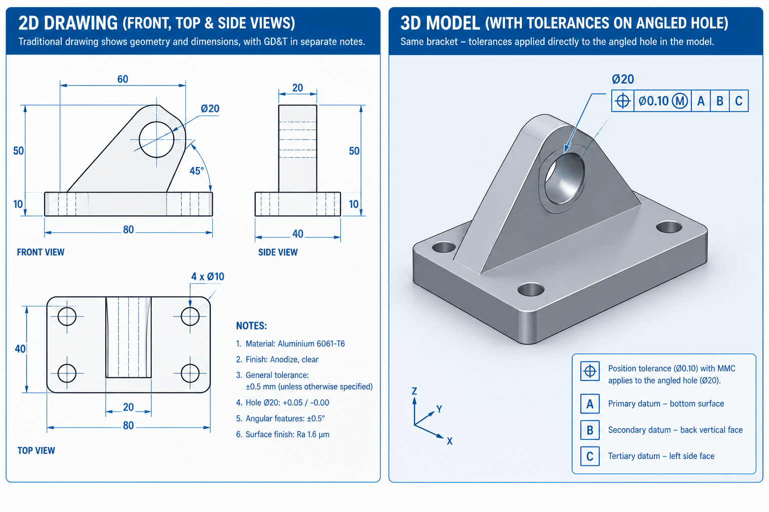
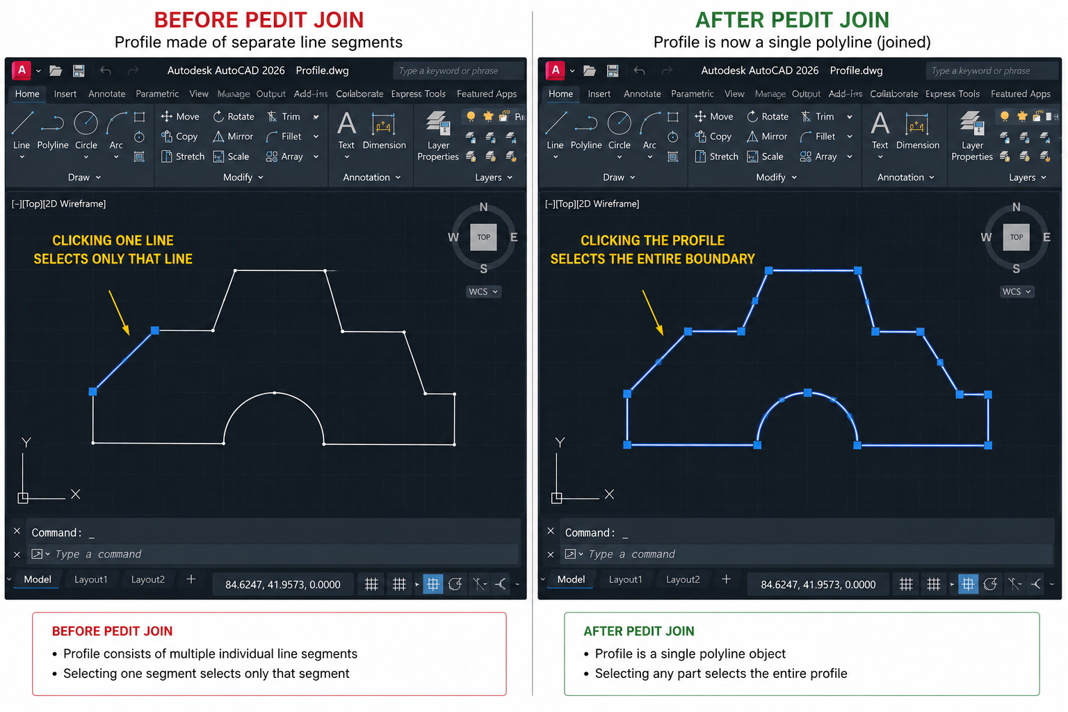
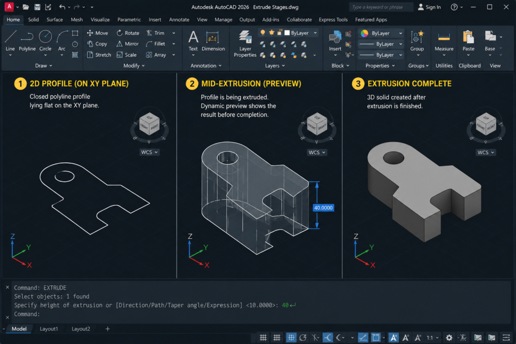
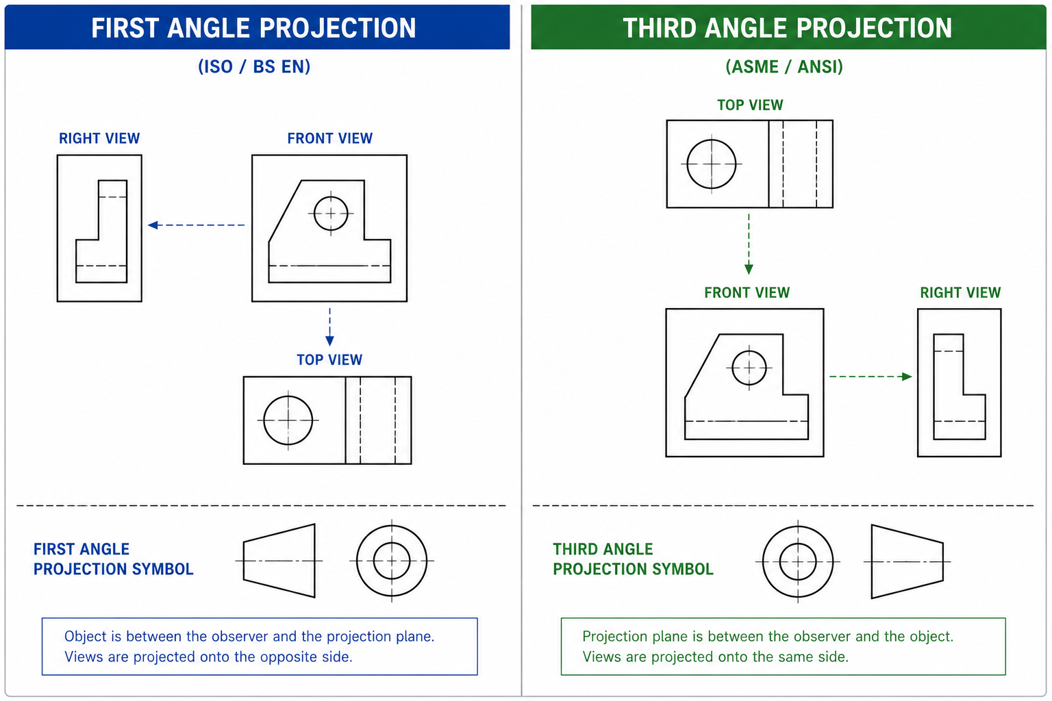
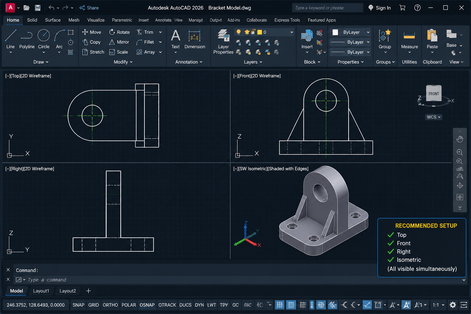
Model-Based Definition (MBD) is a way of defining a part using an annotated 3D CAD model instead of a 2D drawing. The model carries the geometry, dimensions, tolerances and notes in one place, so the 3D model is the single source of truth for design, machining and inspection.
Same part, same tolerances. The only difference is where the information lives.
Why MBD Exists: A Problem 2D Drawings Can’t Fully Solve
Here is a scenario that plays out in real shops. A design change moves a hole. The engineer updates the 3D model correctly. But one of the three views on the drawing still shows the old hole position.
The CNC programmer works from that view. Parts are made to the wrong position. Nobody notices for months, because the shop machined exactly what the approved drawing showed.
The shop did nothing wrong. The process did. Two documents were meant to describe one design, and nothing forced them to stay in sync.
MBD fixes this by removing the second document. There is one model, so there is one place to keep current.
What Is Model-Based Definition, in Plain Terms?
In MBD, the 3D model holds more than shape. It also carries product and manufacturing information (PMI). That includes dimensions, tolerances, GD&T symbols, surface finish, material and process notes.
Each note is attached to the exact feature it describes. A positional tolerance sits on the hole itself, not in the margin of a flat view.
MBD does not make engineering looser or simpler. The same GD&T rules, the same datum logic and the same tolerance discipline apply. What changes is where the information is stored and who, or what, can read it.
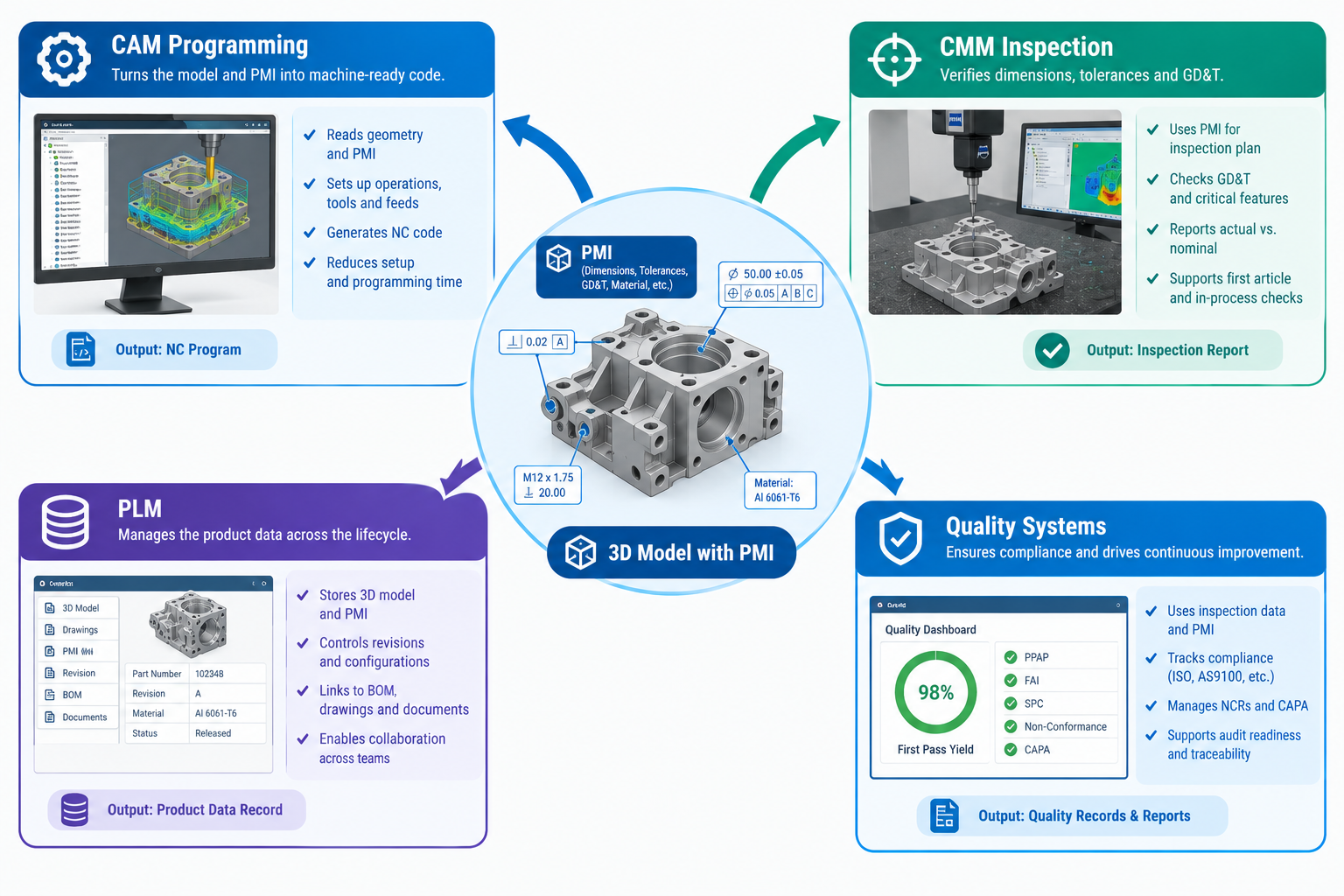
In a drawing, a person reads the note and types it into the next system. In MBD, software such as CAM and CMM programs can read the data directly.
MBD vs 2D Drawings: Key Differences
Aspect
2D drawing-based
Model-based definition
Source of truth
The drawing is legally binding. The 3D model is a reference.
The annotated 3D model is the only binding source.
Where tolerances live
On flat views. The reader rebuilds the 3D shape in their head.
Attached to the 3D feature, viewable from any angle.
Data use downstream
People read the drawing and re-enter data by hand.
CAM, CMM and quality software read PMI directly.
Design changes
Update the model and every drawing view, then check both.
Update one model. Everyone sees the current version.
Complex shapes
Curved or freeform surfaces are hard to define in 2D.
Tolerances attach straight to the curved surface.
Long-term reuse
Someone must re-interpret old drawings.
Structured data can be reused by future tools.
The biggest row is the first one. Once only one document is binding, the sync problem goes away.
What a Complete MBD Dataset Contains
MBD is not “a 3D model with a few dimensions added.” A production-ready dataset has several parts, and each one has a job.
Component
What it holds
Common standard or format
3D geometry
The exact solid or surface shape of the part
Native CAD, or STEP AP242 (neutral format)
PMI
Dimensions, tolerances, GD&T, finish, material and process notes
ASME Y14.41, ISO 16792
Datums and GD&T structure
The reference frame used to measure the part
ASME Y14.5
Saved 3D views
Named, uncluttered views of selected annotations for easy review
Native CAD view tools, 3D PDF
Metadata
Part number, revision, material spec, weight, finish
PLM fields
Inspection data
Characteristics and acceptance criteria that drive CMM programs
QIF (Quality Information Framework)
PMI does most of the work
Geometry alone can’t tell a CAM programmer the tolerance on a hole. It can’t tell a CMM which features to measure either. PMI carries that information.
A 3D model without properly authored PMI is just a reference model. It is not an MBD dataset, no matter how accurate the geometry is.
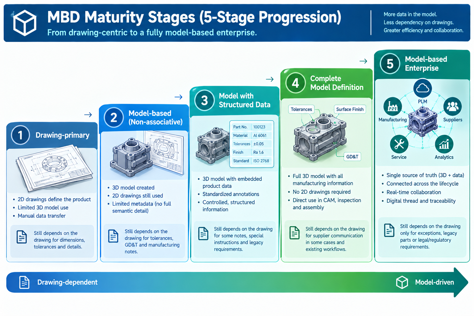
The Five Stages of MBD Adoption
Few companies jump straight from drawings to full MBD. Most move through stages, handing more authority to the model at each step.
Stage
What it means
What still relies on the drawing
1. Drawing-primary
The drawing is the only binding document. The model mainly produces drawing views.
Everything
2. Model and drawing hybrid
Both are controlled. The drawing is still binding. The model is used for CAM and visualisation.
Contract, quality acceptance, and any disputes
3. Model-primary with reference drawing
The annotated model is binding. A simple drawing is made only for partners who can’t use the model yet.
Only external partners not yet equipped for models
4. Model-only (full MBD)
The model is the only deliverable. No drawing is made.
Nothing
5. Model-based enterprise (MBE)
The model feeds a full digital thread across design, planning, quality and support.
Nothing internally
Why Stage 2 is the risky one
Most manufacturers sit in Stage 2. It keeps the main risk of drawings, two documents that can drift apart. It also delivers little of MBD’s benefit, because CAM and CMM programming often still starts from the drawing.
Think of Stage 2 as a stop on the way, not a destination. The opening scenario is exactly what Stage 2 looks like when it goes wrong.
Benefits of Model-Based Definition
The gains are easiest to judge when you tie them to metrics you already track.
Fewer drawing-model mismatches. With one binding source, there is nothing to fall out of sync. Look at nonconformance reports and build-to-wrong-revision incidents.
Faster CAM and CMM programming. Software reads the PMI instead of a person re-typing it. Track programming hours per part.
Fewer misread tolerances on complex parts. Curved and freeform surfaces are easier to define in 3D than in a handful of section views.
Shorter design change cycles. You update one dataset, not a model plus every affected view.
Easier digital manufacturing. Structured data plugs into automation, digital inspection and digital thread systems.
Be realistic about the limits. Benefits only show up when the drawing truly loses its binding status. They also need CAM, CMM and PLM tools that can actually read PMI. And simple prismatic parts gain less than turbine blades, body panels or complex castings.
Where MBD Is Used Today
Adoption varies by industry. It depends on customer pressure, part complexity, volume and traceability rules.
Industry
Why it adopts MBD
Maturity
Aerospace and defense
Prime contractors and government customers require model-based deliverables. Programs run for decades, so structured data has lasting value.
High
Automotive
High volumes and complex body and powertrain shapes.
Moderate to high, strongest at OEMs and Tier 1 suppliers
Medical devices
Strict traceability and tight control of safety-critical dimensions.
Moderate and growing
Electronics and precision instruments
Tiny, dense features are hard to dimension clearly in 2D.
Moderate to high
General industrial equipment
Pressure to cut programming time on high-mix, low-volume work.
Lower to moderate
In defense work, MBD requirements often trace back to MIL-STD-31000 for technical data packages. Aerospace leads because large customers can require MBD from their suppliers. Other industries tend to adopt it from the shop floor up, usually to save programming time.
Common Barriers and How to Handle Them
Barrier
Why it slows things down
What works
Customers and suppliers still want drawings
You end up maintaining both
Use Stage 3 deliberately. Make a reference drawing only when someone truly needs it.
Software and tooling cost
Downstream CAM and CMM tools must read PMI, and staff need training
Start with your most complex or highest-volume parts
Messy 3D annotation
Cluttered PMI is as hard to read as a bad drawing
Set an internal annotation standard with standard views and review checklists
Training gaps
Teams have years of 2D habits
Train each role. Pair new users with experienced mentors.
Long-term file access
Native CAD formats change across versions and vendors
Archive in a neutral format such as STEP AP242 as well
Culture
Experienced staff doubt that a new method is as rigorous
Involve drawing veterans when writing the standard
How to Start With MBD: A Simple Plan
Check your downstream tools first. Find out whether your CAM, CMM and quality software can read PMI. Authoring PMI that nothing consumes gives you almost no return.
Pick a pilot group. Choose your most complex or highest-volume part families. They show the payoff fastest.
Write an annotation standard. Define how PMI is placed, which saved views to use, and how reviewers check it.
Train every role. Designers, programmers, machinists and inspectors all need to read the model.
Retire the drawing’s authority. Make the model binding for the pilot parts. Produce a reference drawing only if a partner needs one.
Measure and expand. Compare nonconformances, programming time and change cycle time against your own baseline. Then move to the next group of parts.
Frequently Asked Questions About MBD
What is model-based definition?
Model-based definition is a method where an annotated 3D CAD model, not a 2D drawing, is the authoritative description of a part. It carries geometry, tolerances, GD&T and notes together. Manufacturing and inspection software can read that data directly.
What is the difference between MBD and a 2D drawing?
A 2D drawing spreads dimensions across flat views, and people must interpret them. MBD attaches the same information to the 3D features and makes it machine-readable. The key difference is authority: in MBD, the model is the only binding document.
What is PMI in MBD?
PMI stands for product and manufacturing information. It covers dimensions, tolerances, GD&T symbols, surface finish and process notes attached to the 3D model. PMI is what CAM and CMM software reads to program machining and inspection.
Can you still make 2D drawings with MBD?
Yes. Many MBD users still make drawings for partners who can’t read models yet. The difference is that the drawing is non-binding and derived from the model. The model stays the only authoritative source.
What software do you need for MBD?
Most major CAD systems, including CATIA, NX, Creo and SolidWorks, can author 3D PMI. The bigger need is downstream: CAM and CMM tools that read PMI, and PLM systems tied to the model. Test those before a wide rollout.
Which standards govern MBD?
ASME Y14.41 covers digital product definition data practices, and ISO 16792 is its international counterpart. ASME Y14.5 covers the GD&T rules used inside the model. Defense programs may also cite MIL-STD-31000.
What is the difference between MBD and MBE?
MBD defines a single part using the model. Model-based enterprise (MBE) extends that model into a digital thread across planning, quality, supply chain and in-service support. MBD is the foundation that MBE builds on.
Conclusion: One Source of Truth Is the Point
The real value of MBD is not nicer 3D software. It is having one authoritative place where design intent lives.
When the model is the only binding document, a drawing can’t silently drift out of date. And when the data is structured, software can use it without anyone re-typing it.
If you are in Stage 2 today, the practical next step is simple. Pick one complex part family, confirm your downstream tools can read PMI, and make the model binding for that group.
For related reading, see our guides on why GD&T matters in high-precision industries, datum selection best practices, tolerance stack-up, digital twin applications in modern engineering and digital twins vs BIM.
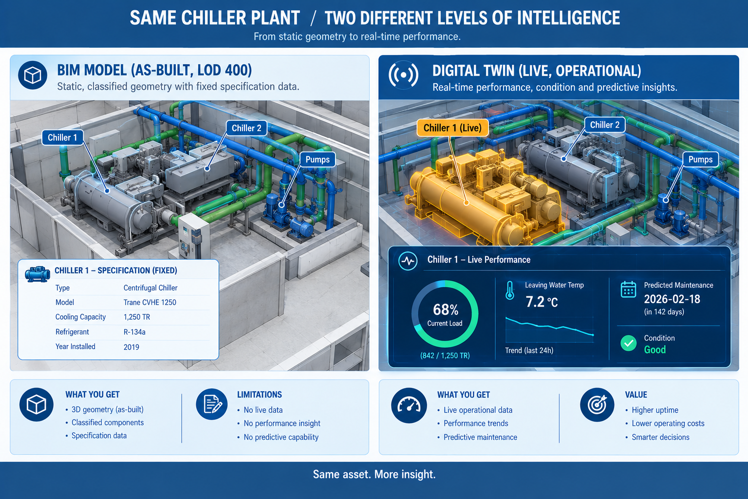
A university’s facilities team, managing a newly completed engineering building, pulled up the project’s handover BIM model to investigate a complaint about uneven temperatures on the third floor. The model showed exactly what it was designed to show: the HVAC system’s design specification, the ductwork layout, and the as-built equipment schedule, accurate as of the day the building was handed over fourteen months earlier.
What it couldn’t show was why the third floor was currently running warm, because the model had no connection to anything happening in the building right now. No current sensor readings, no live equipment status, no record of how performance had drifted since handover. The facilities team’s next step was the same one teams have used for decades: send a technician to manually check dampers, sensors, and control settings floor by floor, a process that took four days to isolate a single miscalibrated VAV box damper that had been slowly drifting out of setpoint since month three.
Quick answer: BIM and digital twins are not competing technologies, and a digital twin is not simply a more advanced or renamed version of BIM. BIM is a static, point-in-time model answering what a building was designed and built to be. A digital twin is a live, continuously updated representation connected to real-time sensor data, answering what a building is actually doing right now, and increasingly, what it’s likely to do next. The most effective digital twins are built directly on top of an accurate BIM model, making the two sequential stages of the same digital representation rather than alternative choices.
This article covers the core differences between BIM and digital twins, the five-stage evolution from a static model to a fully autonomous twin, guidance on when each is the right tool, and worked examples showing the distinction in practice.
Defining the Two Terms Precisely
Building Information Modeling (BIM) is the process of creating and managing a structured, element-based digital representation of a building’s physical and functional characteristics, used primarily to support design, coordination, and construction decision-making. A BIM model is authoritative about design intent and as-built condition: what a building was designed to be, and at LOD 500, what was actually built.
A digital twin, in building and infrastructure contexts, is a live, continuously updated digital representation of a physical asset, connected to that asset through real-time or near-real-time data. This lets the digital representation reflect the asset’s actual current state and, in more advanced implementations, support prediction and even automated control of the physical asset. A digital twin is authoritative about current operational reality.
The two definitions aren’t competing; they describe different relationships between a digital model and physical reality. A BIM model is a snapshot, accurate as of a specific point in time, updated deliberately at defined milestones. A digital twin is a live connection, continuously reflecting whatever the building’s sensors report at this moment.
Six Core Differences Between BIM and Digital Twins
These six dimensions, moving from the most fundamental to the more technical, give a practical picture of how the two actually differ in day-to-day use.
Aspect
BIM
Digital Twin
Example
Primary purpose
Design, document, and coordinate construction, concept through as-built handover
Monitor, analyse, and predict ongoing operational behaviour after occupancy
BIM coordinates ductwork before installation; a twin tracks that same ductwork’s airflow five years into occupancy
Data currency
Represents a point-in-time condition, updated at formal revisions or renovations
Continuously updated with live data, reflecting real-time conditions
BIM shows a chiller’s design spec; a twin shows that chiller’s actual real-time energy draw and fault status
Data direction
One-directional: data flows into the model, little or none flows back out
Bidirectional: sensor data flows in, and in advanced twins, commands flow back out to control systems
A twin can trigger an automatic HVAC adjustment; a BIM model has no mechanism to affect the physical building
Typical lifecycle stage
Concept design through construction and handover, ending at LOD 500
Building operation, often spanning decades after construction
A hospital’s BIM model is finalized at handover; its twin then operates continuously for the building’s 40+ year life
Underlying technology
3D modelling and coordination platforms (Revit, Navisworks)
IoT sensors, real-time data integration, analytics, and increasingly AI/ML, built on a 3D base
A BIM platform manages static model elements; a twin platform manages a continuous stream of sensor readings
Value delivered
Reduces design conflicts, rework, and delays during design and construction
Reduces operational cost, energy waste, downtime, and maintenance inefficiency
The Data Direction Difference Is the Most Consequential
Of these six differences, data direction, one-directional for BIM, bidirectional for a mature digital twin, carries the largest practical consequence. It’s what separates a true digital twin from being simply “BIM with a live dashboard attached.” A monitored twin that only displays live data without acting on it is a valuable but limited tool, essentially a sophisticated visualisation layer. The genuinely transformative applications, automated demand response, self-optimising HVAC control, predictive maintenance that schedules its own work orders, all depend on bidirectional capability that lets the digital representation influence the physical building, not just observe it.
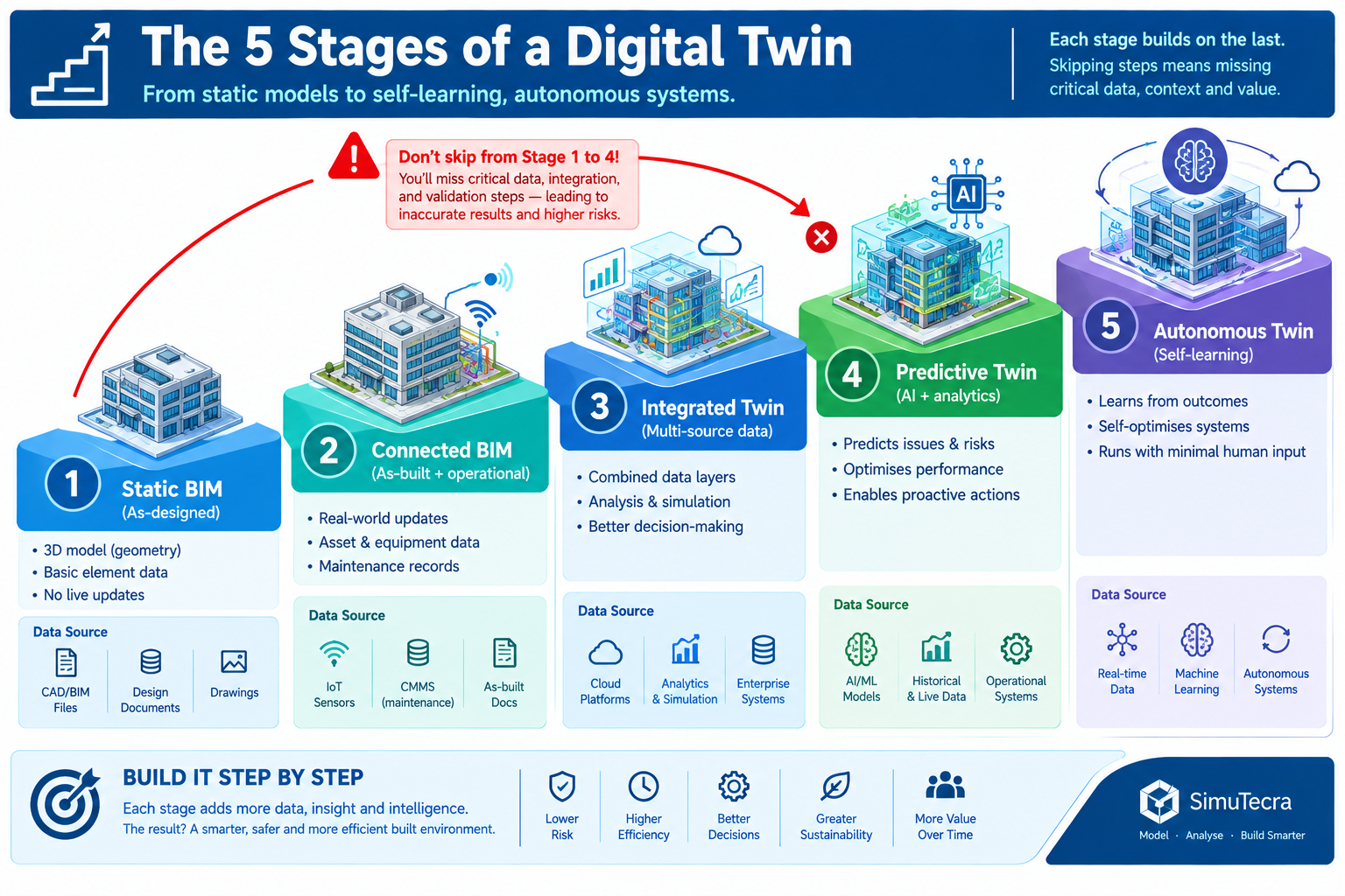
From Static BIM to Autonomous Digital Twin: A Five-Stage Evolution
Most buildings’ digital representations progress through stages, each adding a distinct capability on top of the previous one, rather than making a binary choice between “BIM” and “digital twin.”
Stage
Description
Capability Unlocked
1. Static BIM model
A fixed, element-based model with no live data connection
Design coordination, clash detection, documented as-built record
2. Connected (asset-linked) BIM
The as-built model linked to static asset and maintenance data
Facilities teams locate equipment info directly through the model
3. Monitored digital twin
The connected model linked to live sensor and BAS/BMS data
Live dashboards and alerts when a parameter moves outside threshold
4. Predictive digital twin
Historical data used to build models forecasting future behaviour
Predictive maintenance scheduling and early failure warning
5. Autonomous / prescriptive twin
A live control interface lets the twin issue commands, not just receive data
Automated, continuously optimised building system operation
Why Skipping Stages Rarely Works
Owners occasionally try to procure a predictive or autonomous twin (stages 4 or 5) without first establishing a solid connected BIM foundation (stages 1 and 2), usually because prediction and automation are the most visible part of the pitch. This consistently underperforms, since predictive analytics need historical data accumulated over time, and that data is far more useful tied to accurate, well-classified building elements from a solid BIM foundation than existing as disconnected sensor readings with no spatial or asset context.
The university engineering building shows this dependency directly. The four-day diagnostic process was only shortened by connecting live data to the existing, accurate BIM model of the ductwork and VAV boxes. Without that model as a foundation, live sensor data alone would tell a facilities team a damper was misbehaving without easily showing them where it was or what it connected to.
When BIM Alone Is Enough, and When a Digital Twin Earns Its Cost
Not every building or use case justifies investing beyond a well-executed, connected BIM model.
Use Case
Is BIM Alone Sufficient?
Recommendation
Design coordination and clash detection during construction
Yes, this is exactly what BIM is designed for
Use standard BIM coordination; a twin has no role before the building is operational
Facilities handover and initial asset documentation
Largely yes, with a connected BIM model
Treat a well-structured handover as digital twin readiness, not a full twin
Ongoing energy management and equipment performance monitoring
No, a static model can’t show current consumption or status
Justified for buildings with meaningful energy spend or equipment criticality
Predictive maintenance for critical equipment (chillers, generators, medical equipment)
No, prediction requires historical trend data and analytics
Strongly justified where unplanned downtime carries high cost, like hospitals and data centres
Portfolio-wide space utilisation and occupancy planning
Partially; BIM provides spatial data but not usage patterns over time
Justified for large portfolio owners actively managing space allocation costs
Automated, self-optimising building system control
No, static models have no mechanism to observe or control live systems
Justified only for owners with the operational scale and technical maturity to manage it
Matching Investment to Building Criticality and Scale
The clearest pattern across these use cases: digital twin investment is justified in proportion to how expensive the consequences of not knowing current operational status actually are, and how much scale exists to spread the sensor and platform investment across. A single small office building with modest energy spend has a much weaker case for a predictive twin than a hospital with critical medical equipment and continuous occupancy, or a large campus where the same monitoring platform serves dozens of buildings at once. Size the investment to the specific operational risk and scale of the portfolio, not as a general technology upgrade disconnected from a problem it’s meant to solve.
Worked Examples
A hospital’s critical equipment digital twin: A 400-bed hospital had a complete, accurate BIM model of its central plant and medical gas systems, maintained through several years of minor renovations. Despite the accurate model, the facilities team experienced two unplanned chiller failures in eighteen months, each requiring emergency rental chiller deployment at significant cost, because the existing preventive maintenance programme was based on fixed time intervals rather than actual condition.
The hospital connected its three central plant chillers to a monitored digital twin platform built on the existing BIM model, adding vibration, temperature, and electrical load sensors and feeding that data into an analytics platform trained on historical performance and failure data, reaching stage 4 (predictive) in the evolution above.
Within the first year, the predictive twin flagged a developing bearing wear pattern on one chiller fourteen days before the vibration signature reached the threshold that would previously have gone undetected until failure. This let the facilities team schedule a planned repair during a low-demand period instead of experiencing an emergency failure. The facilities director credited the twin with avoiding at least one of the emergency rental deployments that had cost more than the twin implementation itself.
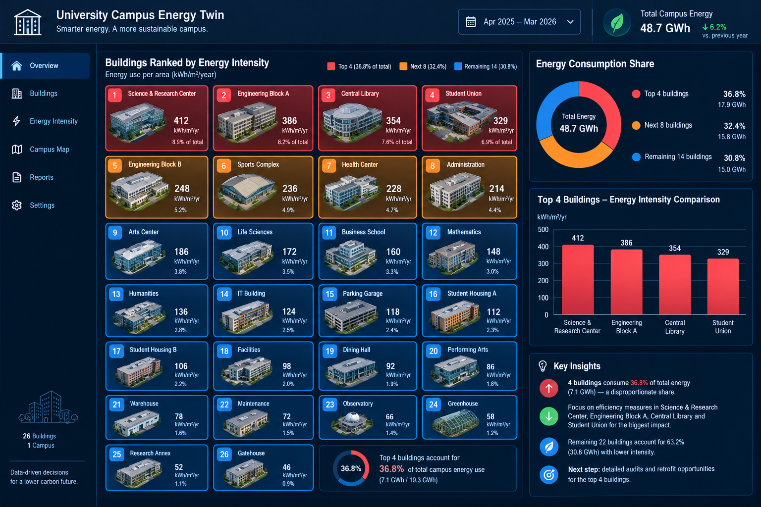
A university campus energy management twin: A university with 26 buildings across its main campus had individually accurate BIM models for each building, produced by different design teams over a 15-year construction programme, but no unified way to compare energy performance across buildings.
The university implemented a campus-wide monitored digital twin (stage 3) that connected each building’s existing utility metering and BAS data into a single platform, using the existing BIM models as the spatial and asset foundation, without initially pursuing predictive or autonomous stages.
The unified live view revealed that four buildings, representing less than 20% of total campus floor area, accounted for nearly 40% of total campus energy consumption, a pattern invisible when each building’s utility data had been reviewed separately with no easy way to compare buildings directly. This directed the university’s capital energy-efficiency investment toward the four highest-consuming buildings first, rather than spreading a limited budget evenly across all 26 regardless of actual need, a targeting decision the static BIM models alone wouldn’t have supported.
Frequently Asked Questions
Can a digital twin exist without a BIM model? Technically yes, a digital twin can be built directly from sensor data or a simplified 3D representation without a full BIM authoring process. For buildings specifically, a twin built on an accurate, element-classified BIM foundation is substantially more useful, since BIM provides the spatial and asset context, which specific duct, which specific chiller, that makes live sensor data meaningful rather than just a stream of unattached numbers.
Does every building need a digital twin? No. The value of a digital twin scales with a building’s operational complexity, criticality, and scale. A well-maintained, connected BIM model is genuinely sufficient for many buildings’ ongoing facilities needs. Small, simple buildings with modest energy spend and no critical equipment often don’t generate enough operational risk to justify the sensor and platform cost.
How much does it cost to move from a static BIM model to a monitored digital twin? Cost varies with building size, how many systems are monitored, existing building automation system capability, and analytics platform sophistication. As a general pattern, a monitored twin (stage 3) is driven primarily by sensor and integration hardware, while a predictive twin (stage 4) adds meaningful software and data science cost on top. Scope a specific pilot, often starting with the highest-value critical equipment, rather than attempting a full-building deployment first.
Is “digital twin” just a marketing term for what used to be called a BMS? There’s real overlap, and some products marketed as digital twins are, in substance, a building management system or CMMS with a 3D visualisation layer added. The meaningful distinction is whether the platform is genuinely connected to an accurate, element-level 3D model derived from BIM, and whether it supports the predictive or bidirectional-control capabilities described above, rather than only displaying current sensor readings on a floor plan.
Who should own a digital twin implementation within a facilities organisation? This typically sits with the facilities management or operations team, since a digital twin is fundamentally an operational tool, but it should be planned in coordination with whoever managed the original BIM delivery to ensure the foundation is accurate and well-classified. Larger or more technically ambitious programmes, particularly those pursuing predictive or autonomous capability, often add a dedicated data or analytics role, since building and maintaining predictive models requires data science skills traditional BIM or facilities roles don’t typically include.
Key Takeaways
The university engineering building had an accurate BIM model and still spent four days manually diagnosing a problem a monitored digital twin would have flagged within days. The hospital and campus examples show what changes when a live, data-connected layer is added on top of an accurate model foundation: not a replacement for BIM, but a genuinely new capability a static model, however accurate, was never designed to provide. In every case, the BIM model remained useful and necessary, both as the design and construction record and as the foundation the digital twin was built on.
This is the relationship worth remembering past the terminology: BIM answers what a building was designed and built to be, and a digital twin answers what that building is actually doing right now and, at its most capable, what it’s likely to do next, consistent with the maturity framework defined by the Digital Twin Consortium. Neither replaces the other, and the strongest operational outcomes came from treating the digital twin as the next stage built on a solid BIM foundation, not as a competing technology chosen instead of one.
Owners and facilities teams evaluating this decision are best served by being precise about which of the five evolution stages their building currently occupies, and which specific operational problem the next stage of investment would actually solve, rather than pursuing “a digital twin” as an undifferentiated technology goal disconnected from the operational reality their facilities team is actually managing day to day.
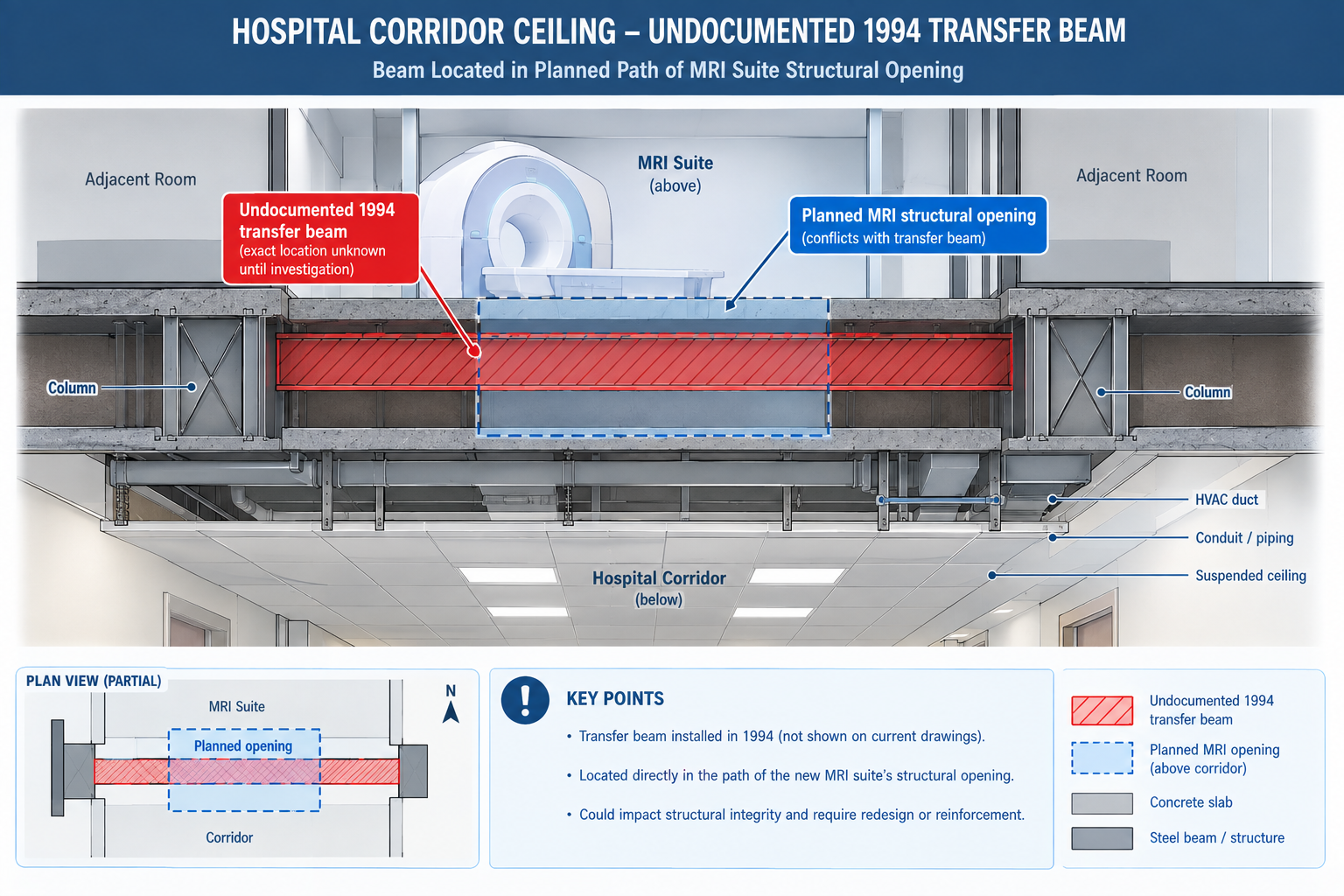
A regional health system planning a major renovation of a 1970s-era hospital wing commissioned the design based on the building’s original architectural drawings, supplemented by a handful of field measurements taken during a walkthrough.
Three weeks into demolition, the contractor discovered a section of corridor ceiling concealed a structural transfer beam that appeared nowhere in the drawings. It had been installed during an unrecorded 1994 renovation to support a rooftop mechanical unit added at that time. The beam sat directly in the path of a new MRI suite’s structural opening, already planned and approved.
Quick answer: The discovery halted demolition for eleven days while a structural engineer assessed the beam, the design was revised around it, and the revision was resubmitted for approval. On an active hospital renovation that had to stay partially operational throughout construction, that delay carried significantly higher cost and disruption than it would have on a vacant building. The beam had been there the entire time. What was missing was a reliable way to capture it before the design was finalised. That’s the gap scan-to-BIM closes: converting a building’s true, current physical condition into an accurate 3D model the design team can trust, instead of relying on original drawings that quietly stopped matching reality years earlier.
This article covers the reality capture technologies used to gather existing-conditions data, the six-stage scan-to-BIM process, the benefits specific to renovation and facilities projects, what drives project cost, and worked examples in practice.
What Scan-to-BIM Actually Is
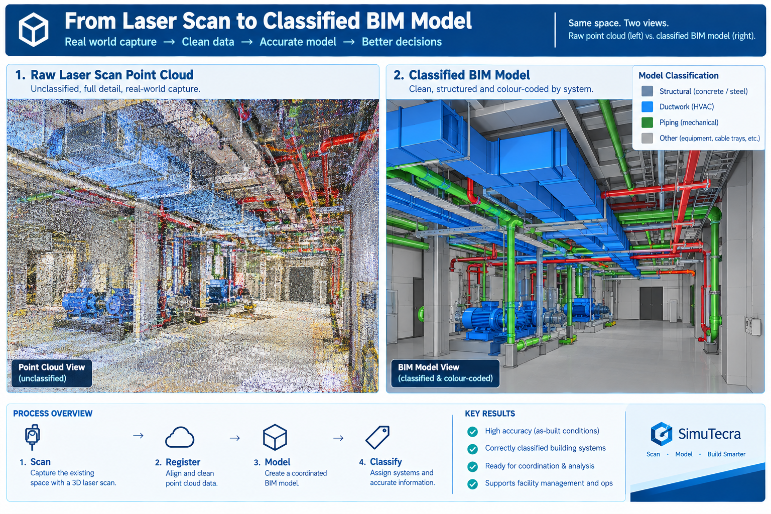
Scan-to-BIM captures a building’s existing physical condition using 3D reality capture technology, most commonly laser scanning, and converts that data into a structured Building Information Model a design or facilities team can use the same way they’d use a model authored from scratch. The output isn’t the raw scan itself, a point cloud of millions of individually measured 3D points, but a modelled interpretation of it: walls, structure, and MEP systems traced and classified into an organised, element-based model.
The point cloud and the finished model serve different purposes, and a complete deliverable should include both. The point cloud is the unfiltered record of physical reality, every visible surface at true measured accuracy, with no interpretation applied. The finished model is an interpreted simplification built to a defined level of development, so it can be federated and clash-tested using standard BIM workflows. Keeping the point cloud alongside the finished model lets anyone downstream independently verify what the model claims about a specific area, exactly the kind of check that would have caught the concealed hospital beam before, not after, demolition began.
The Reality Capture Technologies Behind Scan-to-BIM
Choosing the wrong technology for a given scope is one of the most common sources of both cost overrun and accuracy shortfall.
Technology
Typical Accuracy
Capture Speed
Best Suited For
Terrestrial laser scanner (tripod)
2-5mm at building-interior range
Slower per setup (2-8 min); many setups for full coverage
The Scan-to-BIM Process: Six Stages From Scope to Handoff
Scan-to-BIM is a structured production process, not a single scanning visit. The finished model’s quality depends as much on the planning and verification stages around the scan as on the technology itself.
Stage
What Happens
Common Pitfall
1. Scope definition and scan planning
Define required accuracy, target LOD, which systems to capture, and the technology mix
Scoping without confirming what the model will actually be used for, causing over-capture or missing detail
2. Field data capture
Crews capture the site, placing control points to tie scans into a consistent coordinate system
Insufficient overlap or control points, leaving gaps or accuracy drift expensive to fix later
3. Registration and point cloud processing
Individual scans are aligned into a single, unified, cleaned point cloud
Accepting a registered point cloud without verifying it against control points, letting errors propagate
4. Model authoring to target LOD
Modellers build the BIM model from the point cloud to the agreed level of detail
Modelling every visible feature indiscriminately instead of to the agreed LOD, producing an oversized, expensive model
5. Quality assurance and accuracy verification
The model is checked against the point cloud and survey control for accuracy and completeness
Skipping independent QA and relying solely on the modelling team’s self-review
6. Deliverable handoff and integration
The model, point cloud, and documentation are delivered and integrated into the project workflow
Delivering the model without the point cloud or QA documentation, leaving the client unable to verify it later
Why Scope Definition Is the Highest-Leverage Stage
Scope definition carries disproportionate weight because it sets the target accuracy and LOD every later stage is measured against. A scope specifying survey-grade accuracy and LOD 350 detail where LOD 200 general planning would suffice spends far more than the project needs. A scope that under-specifies LOD for a project that actually needs coordination-ready detail delivers a model that looks complete but can’t support the workflow the design team needs, forcing a costly re-scope later.
The hospital renovation illustrates getting scope wrong in the other direction. Relying on original drawings and a walkthrough, rather than commissioning any capture at all, is itself a scope decision, one assuming the drawing record was reliable enough to design from directly. For buildings with any unrecorded modification history, that assumption is very often wrong.
The Benefits of Scan-to-BIM, and Where Each One Applies Best
Scan-to-BIM’s benefits concentrate on projects where existing conditions matter and can’t be fully trusted from drawings alone.
Benefit
Mechanism
Best Suited Project Type
Accurate existing conditions for renovation design
Captures true, current geometry instead of relying on outdated or missing drawings
Renovation, retrofit, and adaptive reuse, especially buildings older than 20-30 years
Reduced field verification trips
A complete point cloud eliminates repeated site visits to manually verify conditions
Design teams not co-located with the site, or restricted-access sites
Faster and more reliable design coordination
The as-built model can be clash-tested against new design elements like any discipline model
Renovation projects coordinated using a full BIM workflow
Reduced construction rework from unknown conditions
Conflicts with undocumented existing structure are caught in the model, not by a demolition crew
Any renovation, especially in occupied or operational buildings
Reliable facilities management and space planning data
Gives facilities teams a verified baseline for maintenance and future capital planning
Large portfolios without reliable current documentation
Connecting Scan-to-BIM to the Rest of the Coordination Workflow
A scan-to-BIM model delivers the most value when it’s not treated as a standalone deliverable but federated into the same coordination workflow used for new design: brought into the common data environment as the authoritative existing-conditions reference, clash-tested against new elements, and maintained through construction like an as-built model. Renovation projects that integrate the scan into a full coordination programme capture the benefit twice, once from the accuracy of the capture itself, and again from standard BIM coordination benefits, fewer RFIs, less rework, more reliable scheduling, now extended to a project that would otherwise have had no reliable existing-conditions model at all.
What Drives Scan-to-BIM Project Cost
Cost varies widely by project. A meaningful quote depends on the specific combination of these factors rather than a single per-square-foot number.
Cost Factor
Description
Why It Varies
Building size and site complexity
Total floor area and physical complexity, often the single largest cost driver
Open, simple spaces need fewer scan setups per unit area than congested, MEP-dense spaces
Required accuracy and LOD
Higher accuracy and target LOD need slower scanning and significantly more modelling time
Modelling time scales non-linearly with LOD; each added level needs proportionally more verification
Site access and operating conditions
Occupied, hazardous, or restricted sites slow field capture and may need off-hours scanning
Restricted access reduces effective scanning hours per day and adds safety/escort requirements
Element categories and system detail required
Architectural-only versus full MEP-inclusive scope with ductwork and piping modelled
MEP systems are geometrically dense and often partially concealed, needing more careful interpretation
Deliverable format and software compatibility
The required authoring platform, classification standard, and integration needs
Providers experienced with a client’s specific platform work faster than those adapting for the first time
Weighing Scan-to-BIM Cost Against the Cost of Not Doing It
The more consequential comparison for most project decisions is against the cost of proceeding without a scan, relying on outdated drawings and field measurement, as the hospital renovation did. The eleven-day delay from the concealed beam, on an occupied hospital renovation, almost certainly cost more than a full scan of the affected wing would have. That comparison typically holds for any renovation of meaningful scope: weigh the cost of scan-to-BIM against the cost of the specific field discoveries and redesigns it’s likely to prevent, not as a standalone expense. Buildings with a long, undocumented modification history are where this comparison most reliably favours commissioning the scan.
Worked Examples
A historic theatre renovation: A 1920s-era theatre undergoing a seismic retrofit and accessibility renovation had no reliable original drawings, having been renovated at least four times with no consistent as-built record surviving. The retrofit design depended on knowing exactly how the existing structure was configured, not an assumed condition.
The project commissioned a terrestrial laser scan of the entire building, prioritising survey-grade accuracy for the seismic engineering use case, combined with drone photogrammetry of the exterior facade and roof. The point cloud was modelled to LOD 300 for structural elements and LOD 200 for architectural finishes not relevant to the seismic scope, a deliberately mixed-LOD approach matched to how each part would actually be used.
The scan revealed that a section of the original timber roof structure had been partially reinforced with steel during an undocumented 1960s repair, a condition the structural engineer needed to correctly model the existing structure’s seismic behaviour. Designing the retrofit without this information risked a design that misjudged the structure’s actual capacity. The scan-to-BIM model became the structural engineer’s primary reference for the entire retrofit, replacing the unreliable drawing record entirely.
A manufacturing facility equipment relocation: A manufacturing company relocating a production line within an existing 1980s facility needed to verify that new equipment, with specific clearance requirements, would fit within an existing bay alongside structural columns, overhead crane rails, and utility routing, none of it documented in drawings that predated at least three prior equipment changes in the same bay.
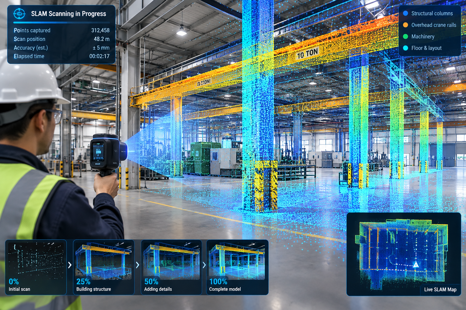
A handheld SLAM scan captured the full production bay in under two hours, prioritising speed over survey-grade accuracy since the use case was equipment fit and clearance checking, not structural design. The point cloud was modelled to LOD 200-300, sufficient to run a clearance check without the cost of a survey-grade capture the project didn’t need.
The clearance check identified that the new equipment’s largest component wouldn’t clear an existing overhead crane rail bracket by the margin the manufacturer’s installation requirements specified, a conflict invisible in the facility’s outdated drawings, which didn’t reflect the bracket’s actual as-installed position after a prior modification. Catching the conflict before equipment delivery let the facility relocate the bracket during a scheduled maintenance window rather than during the tightly scheduled production line changeover, avoiding unplanned downtime.
Frequently Asked Questions
How accurate does a scan-to-BIM model need to be?
It depends on the use case. Structural or seismic engineering, precision MEP coordination, and historic preservation typically need survey-grade accuracy (a few millimetres) from terrestrial laser scanning. General space planning and equipment clearance checks often only need 10-30mm accuracy, achievable faster with handheld SLAM scanning. Define the required accuracy before selecting the technology, rather than defaulting to the highest accuracy available.
Can scan-to-BIM be used for an entire building, or only specific areas?
Both are common. A full-building scan fits a renovation spanning the whole building or an owner wanting a complete facilities record. A targeted scan of specific floors or systems fits a limited project scope, like the manufacturing example here. Scoping the capture area precisely to what’s needed is one of the most effective ways to manage cost without sacrificing accuracy.
How long does a typical scan-to-BIM project take from field capture to finished model?
Field capture is often the fastest stage, from a single day for a small space to several weeks for a large or access-restricted building. Registration, modelling, and QA typically take substantially longer, often several times the field capture duration, since modelling to a coordination-ready LOD is a detailed manual process. Confirm the modelling and QA timeline with the provider based on the specific scope and target LOD.
Is scan-to-BIM only useful for renovation projects, or does it have a role in new construction too?
It has a role in new construction as well: capturing as-built structural or MEP work before it’s concealed by later construction, verifying fabricated components match design models within tolerance, and documenting final as-built conditions for facilities handover. The core value, replacing an assumed condition with a verified, measured one, applies any time there’s meaningful uncertainty about what’s actually built or what exists.
What should a client look for when selecting a scan-to-BIM provider?
Look for experience with the specific scanning technology the project needs, since not every provider is equally strong across terrestrial, SLAM, and photogrammetry capture. Check for a documented accuracy verification process, ideally a QA report comparing the model against survey control. Confirm they’ll deliver the underlying point cloud alongside the finished model, not just the model itself, so the accuracy can be independently verified.
Key Takeaways
The concealed hospital beam, the undocumented theatre reinforcement, and the relocated crane rail bracket share a common thread: each was a physical condition that existed on site, invisible in the available drawings, found either expensively during construction or affordably during design depending on whether the project had commissioned an accurate capture beforehand. None of these discoveries needed unusual diligence to catch once a scan-to-BIM model existed; each was a straightforward measurement once the building’s true condition was actually captured rather than assumed from a drawing record that had quietly stopped being accurate.
This is the core case for scan-to-BIM on any project involving an existing building. Original drawings and even careful field measurement can’t reliably substitute for a systematic, verified capture of current conditions, particularly for buildings with any undocumented modification history, which describes the large majority of buildings more than a decade or two old, a gap the reality capture guidance in the GSA BIM Guide for 3D Imaging was specifically developed to address for institutional projects.
The six stages covered here, scope, capture, registration, modelling, QA, and handoff, exist to convert that physical reality into a model reliable enough to design and coordinate against, with the same confidence a design team would have working from a model of a building that doesn’t yet exist.
Weighed against the cost of the field discoveries, redesigns, and schedule delays it prevents, scan-to-BIM is rarely the most expensive line item on a renovation budget. It’s one of the more reliable ways to make sure the rest of that budget is spent designing and building against what’s actually there, rather than against what an old drawing set assumed still was.
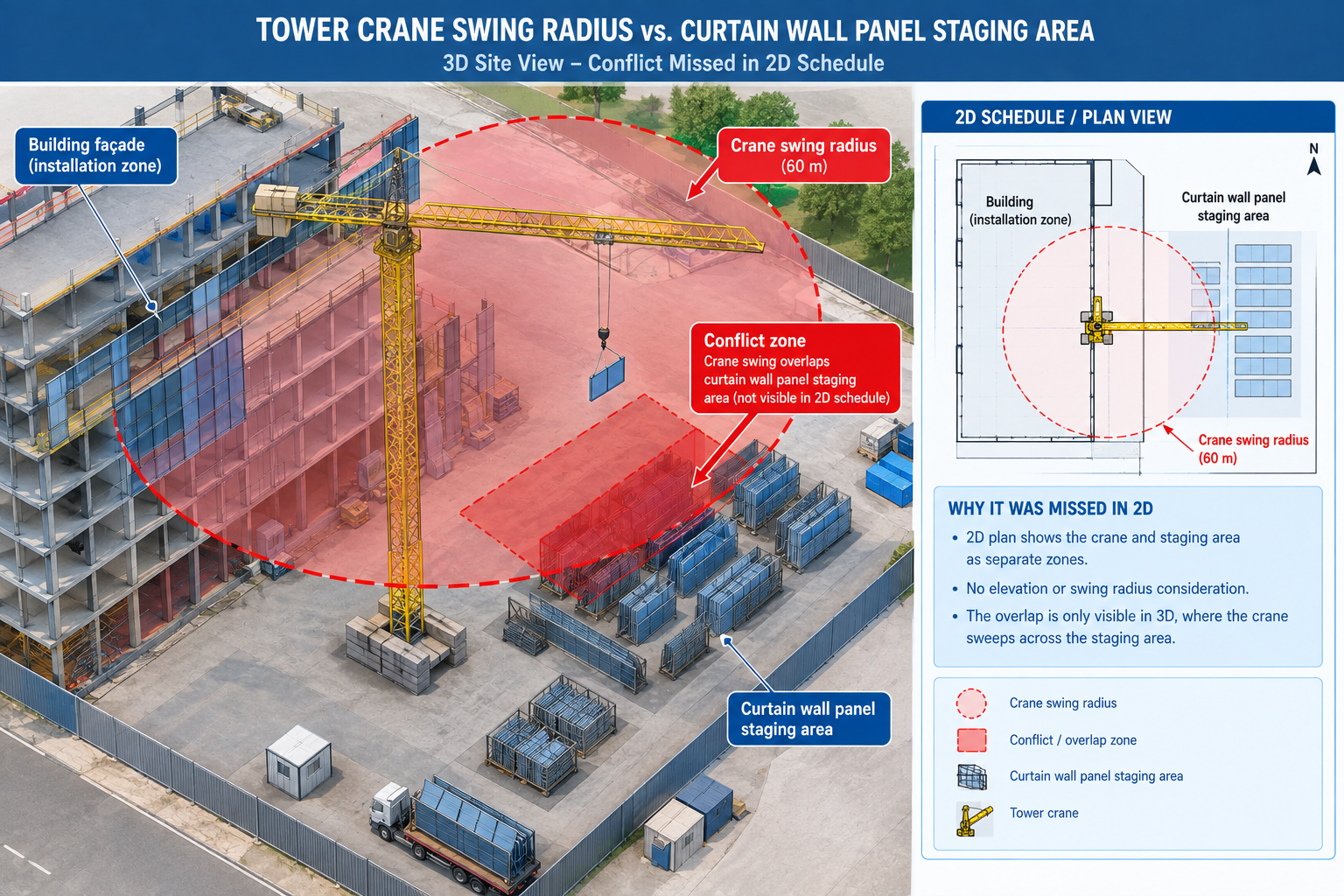
A 22-storey mixed-use tower was seven months into structural erection when the general contractor’s superintendent discovered that the tower crane’s planned swing radius for lifting curtain wall panels to the sixth floor would sweep directly through the staging area where those same panels were scheduled to be stored before installation. Two activities, each individually scheduled correctly, had never been checked against each other in three dimensions.
The schedule, built and maintained in a standalone scheduling tool with no link to the building model, showed both activities happening the same week because that week’s sequence looked correct on paper: steel substantially complete, curtain wall crew mobilised, crane available. Nobody had checked whether the crane could physically reach the panels without its swing path crossing the space where the panels themselves were sitting.
Quick answer: The conflict cost eleven days: four to identify a temporary alternate staging location, three to renegotiate the crane’s lift sequence with the steel erector, and four of lost curtain wall progress implementing the new sequence. Every individual activity in the original schedule had been logically planned. What was missing wasn’t planning discipline; it was a way to test the plan against the physical, three-dimensional reality of the site before committing crews and equipment to it. This is what BIM does for delay prevention: it’s not one tool that fixes delays generally, but a set of distinct methods, each targeted at a specific delay mechanism, from clash detection for physical conflicts to 4D simulation for sequencing conflicts.
This article covers the six most common causes of construction delay, the specific BIM dimensions and methods that address each one, the six-stage process for implementing BIM in a way that actually prevents delays, and two worked examples showing the argument in practice.
The Six Most Common Causes of Construction Delay, and What BIM Does About Each
Construction delays rarely have a single cause; they accumulate from recurring, well-understood problems that appear on nearly every project. What varies is how early each is caught and how disruptive the fix is once found.
Delay Cause
Description
Typical Schedule Impact
BIM Method / Tool
Design conflicts discovered on site
2D drawings didn’t reveal a physical overlap between systems before construction
1-4 weeks per major conflict
3D clash detection (Navisworks, Solibri) run on a recurring cycle through design
Inaccurate or incomplete quantity take-offs
Manual take-offs from 2D drawings are wrong, causing late reorders or oversupply
1-3 weeks per major shortfall
5D BIM quantity take-off and cost estimating tools, model-linked and auto-updating
Unclear or outdated construction sequence
The site team works from a static schedule that doesn’t reflect design evolution
1-6 weeks cumulative from repeated resequencing
4D BIM scheduling simulation, schedule linked directly to model elements
Late or unresolved RFIs
Design ambiguities aren’t caught until a subcontractor in the field can’t proceed
3-15 days per RFI cycle, multiplied by stalled critical-path work
Federated model as a common reference; cloud-based CDE for RFI tracking
Model-based fabrication with digital model handoff, bypassing 2D shop drawings
Poor stakeholder communication and approval delays
Owners, architects, and contractors interpret drawings differently
1-4 weeks per major disagreement
Cloud-based model viewers and common data environments for real-time shared visualisation
Why RFIs Are the Clearest Early-Warning Signal
Among these six causes, the volume and cycle time of requests for information (RFIs) deserves particular attention, since it’s the delay mechanism most directly visible in ongoing project data, long before the delay itself shows up in the schedule. An RFI is, by definition, a moment where the field can’t proceed without clarification, and every day it stays open is a day the affected activity, and often activities scheduled after it, can’t move forward with certainty. Projects that track RFI volume and cycle time as a leading indicator, rather than only reviewing schedule variance after the fact, can catch a coordination breakdown while it’s still a paperwork problem rather than a field delay.
A shared, coordinated 3D model reduces RFI volume by resolving underlying ambiguity before construction reaches that point, and reduces RFI cycle time for the RFIs that still occur by giving the responding party an exact model location and geometry to reference rather than a written description requiring back-and-forth clarification. Both effects compound: fewer RFIs, each resolved faster, is a meaningfully different schedule risk profile than a project relying on 2D drawings alone.
The BIM Dimensions That Do the Delay-Prevention Work
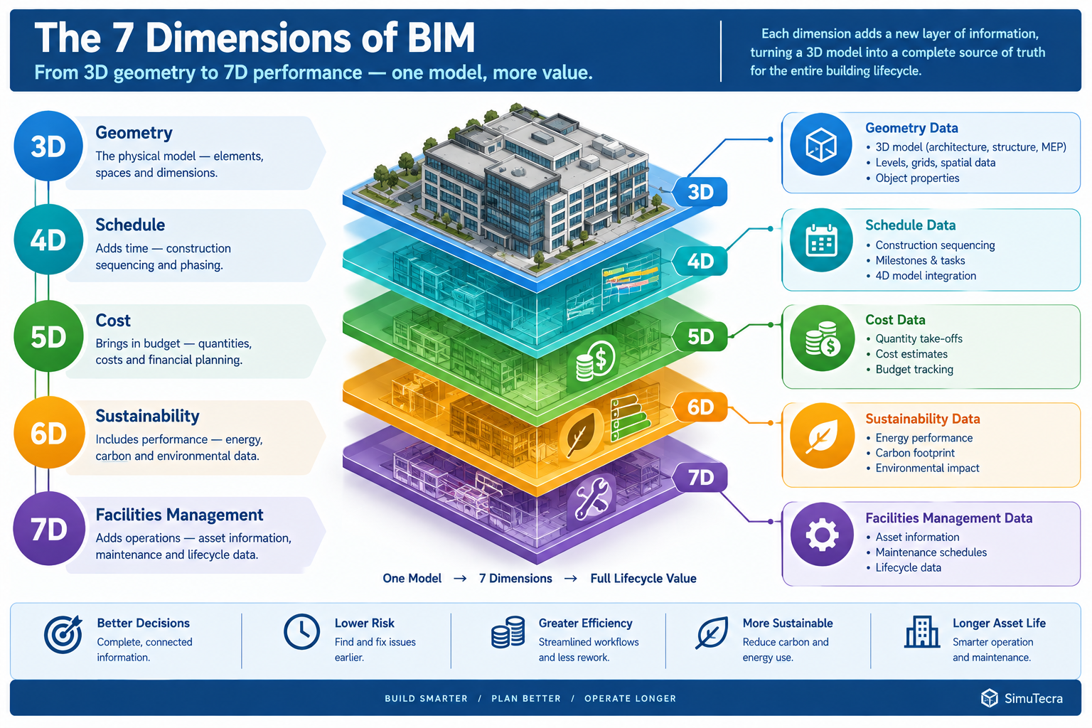
The “dimension” numbering (4D, 5D, and so on) is more convenient shorthand than a strict technical hierarchy, but each does correspond to a distinct type of data linked to the model and a distinct delay-prevention mechanism.
BIM Dimension
What It Adds
Delay-Prevention Mechanism
Representative Tools
3D, Geometry
Three-dimensional representation of every building element from every discipline
Makes physical conflicts visible before construction, replacing flat 2D overlay review
Revit, ArchiCAD, Tekla Structures
4D, Schedule
Schedule activities linked directly to model elements
Reveals sequencing conflicts, an element scheduled before its access route or preceding trade is complete, before it reaches the field
Navisworks TimeLiner, Synchro
5D, Cost
Cost data linked to model elements, auto-updating as design changes
Prevents late-discovered budget overruns from triggering mid-construction redesign scope cuts
Autodesk Assemble, CostX, Vico Office
6D, Sustainability
Energy and sustainability data linked to elements
Prevents late-stage code or certification compliance failures requiring redesign after construction starts
Autodesk Insight, IES Virtual Environment
7D, Facilities management
Asset and maintenance data linked to elements for post-construction use
Reduces commissioning delays from incomplete or inconsistent handover documentation
FM:Systems, Archibus, Autodesk Tandem
4D Scheduling: The Dimension Most Directly Tied to Delay Prevention
Of these dimensions, 4D scheduling aims most directly at delay prevention, since it’s the only one that tests the time dimension of the project against the model rather than cost, sustainability, or facilities data. The tower crane conflict is a canonical 4D problem: two activities correctly scheduled in isolation created a physical conflict only visible when their spatial footprint was checked against each other during the same time window. A 4D simulation run before the schedule is finalised, and re-run as the schedule and design evolve through construction, catches exactly this category of conflict before crews, equipment, and materials commit to a sequence that can’t physically work.
The practical value of 4D simulation depends heavily on keeping it current. A 4D model built once at project kickoff provides a useful early check but a false sense of security later if not updated as both the schedule and design continue to change. Projects that treat 4D simulation as a living tool, updated on the same recurring cycle as clash detection, catch sequencing conflicts throughout construction rather than only at the outset.
Implementing BIM for Delay Prevention: A Six-Stage Process
Owning BIM software, or even having each discipline produce a 3D model, doesn’t by itself prevent delays. The delay-prevention benefit comes from a disciplined process built around the model.
Stage
Activity
Common Pitfall
1. BIM execution planning
Define BIM goals, level of development requirements, model ownership, and specific delay-prevention uses before design begins
Treating the BEP as a compliance formality that’s signed but not actually followed
2. Model authoring and federation
Each discipline authors to the agreed detail level and federates into a shared environment on a recurring cycle
Inconsistent levels of detail across disciplines, hiding conflicts because one discipline hasn’t modelled that scope yet
3. 4D schedule linking
Schedule activities are linked to model elements and simulated to check access, logistics, and sequencing before the schedule is finalised
Building the simulation once at kickoff and never updating it as schedule and design evolve
4. Ongoing coordination and clash resolution
Clash detection continues on a recurring cycle through design and into early construction
Coordination slowing or stopping once construction starts, even though field conditions keep generating new conflicts
5. Fabrication and construction model handoff
Model geometry hands off directly to fabricators rather than being redrawn into 2D shop drawings
Fabricators working from an outdated model version due to unclear version control
6. Facilities handover and closeout
The as-built model, updated with field-verified changes, is delivered to the owner with asset and maintenance data
Deferring model updates until the end, producing a rushed, incomplete as-built model
The BIM Execution Plan: Where Delay Prevention Is Won or Lost
The first stage is disproportionately important because it defines whether the remaining five are actually structured to prevent delays or are simply producing a coordinated model as a documentation exercise. A BIM execution plan (BEP) that specifies model federation and clash detection but not 4D schedule linking will catch physical conflicts but miss sequencing conflicts of exactly the kind that delayed the tower crane example.
A BEP that doesn’t specify how the as-built model will be maintained through construction will produce a coordinated design model but a facilities handover gap at project close. Each specific delay-prevention use, clash detection, 4D sequencing, quantity take-off, fabrication handoff, facilities data, should be explicitly scoped in the BEP, since a model built without a defined use for a specific benefit rarely delivers that benefit by accident.
Measured Benefits: Where BIM’s Delay Reduction Shows Up in Project Data
Rather than treating “BIM reduces delays” as a single unmeasurable claim, each benefit ties to a specific project metric a scheduler or owner would already be tracking.
Benefit
Mechanism
Where It Shows Up
Caveats
Fewer schedule-impacting RFIs
Geometric ambiguities resolved in the coordinated model before construction
RFI logs and critical-path variance reports
Largest for MEP-heavy, congested-space projects; smaller relative benefit for simpler projects
Reduced rework and change orders
Conflicts caught in the model fixed as design changes rather than field improvisations
Change order logs and field rework tracking
Savings depend on how disciplined the resolution and verification process actually is
Faster procurement and fabrication cycles
Accurate, model-derived quantities shorten time from design finalisation to delivery
Procurement lead-time tracking and fabrication schedule adherence
Depends on trade contractors’ own fabrication capability and willingness to work from model data
More reliable schedule commitments
4D simulation identifies conflicts before the schedule is issued
Schedule variance reports and revision frequency during construction
Simulation quality depends on how current the underlying model and schedule data are
Shorter commissioning and closeout
Accurate, continuously updated as-built model reduces documentation gaps
Commissioning schedule adherence, substantial-to-final completion gap
Requires the owner’s facilities team to have systems in place to actually use the handover data
Why the Benefit Is Concentrated in Complex, Multi-Trade Projects
The delay-reduction benefit isn’t uniform across project types; it scales with the density of interdependent systems and trades, since that density determines how many opportunities exist for the kind of conflict BIM catches. A single-storey warehouse with a simple structural system and minimal MEP scope has relatively few opportunities for a tower-crane-style sequencing conflict or ceiling-void congestion, so the absolute delay-prevention benefit of a full BIM programme is smaller, even though the underlying methods still apply.
A hospital, laboratory, or high-rise mixed-use tower, with dense, interdependent MEP systems, tight sequencing, and multiple concurrent trades in the same physical space, is where the benefit concentrates most heavily, since those are exactly the conditions under which 2D-only coordination is least reliable.
Worked Examples
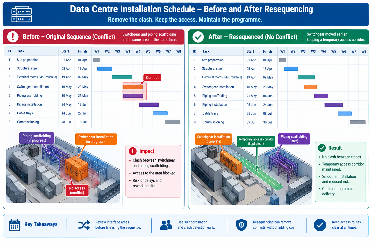
A data centre fit-out schedule: A hyperscale data centre fit-out had an aggressive 34-week schedule driven by a fixed equipment delivery date, with cooling infrastructure, electrical switchgear, and server rack installation sequenced to overlap heavily in the same rooms. The original schedule, built in a standalone tool by an experienced scheduler, showed a logically sound sequence with appropriate lead and lag times.
When linked to the coordinated model and simulated in 4D, the simulation revealed that the electrical switchgear installation crew, scheduled for weeks 18 through 21, would need access to a room that the cooling infrastructure crew’s overhead chilled-water piping, scheduled for week 17, would already have enclosed with scaffolding and temporary bracing blocking the switchgear’s only practical delivery path.
The simulation gave the team six weeks of advance warning, time to resequence the chilled-water piping installation to leave a temporary access corridor open until the switchgear was delivered and positioned, then complete the remaining piping afterward, a one-day schedule logic change made in the office. This avoided what the team estimated would otherwise have been a two-to-three week delay bringing in additional rigging equipment to manoeuvre the switchgear around completed piping and scaffolding, a delay that would have directly threatened the fixed equipment delivery date the entire schedule was built around.
A renovation project with unknown existing conditions: A hospital renovation involved gutting and rebuilding three floors of an operating 1980s-era building while adjacent floors stayed occupied and in clinical use. The original design was based on the building’s archived 2D drawings, known to be incomplete and, in places, inconsistent with the building’s actual as-built condition after four decades of undocumented modifications.
The project team commissioned a 3D laser scan of existing conditions before finalising the renovation design, converting the point-cloud data into an as-built 3D model capturing the building’s true existing structure, ductwork, and piping routes, rather than relying on archived drawings. The new design was then coordinated directly against this verified as-built model.
Scan-based coordination identified 47 locations where the building’s actual condition differed materially from the archived drawings, including a structural beam relocated during a 1990s renovation, reflected in no drawing set, that would have directly conflicted with a new mechanical shaft location in the original design.
Because these discrepancies were identified against a verified model before construction began, the design was adjusted in the office rather than discovered by a demolition crew mid-renovation, in an occupied hospital where an unplanned structural or MEP discovery carries especially high schedule and safety risk. The team credited the upfront scanning investment with avoiding an estimated several weeks of cumulative delay that unknown existing-condition conflicts would otherwise have caused across the renovation’s three floors.
Frequently Asked Questions
Does BIM eliminate construction delays entirely?
No single method eliminates delays entirely, since some causes, weather, material supply chain disruption, labour availability, sit outside what a coordinated model and schedule simulation can address. BIM’s delay-prevention benefit concentrates specifically in the categories covered here: design conflicts, sequencing conflicts, quantity and procurement errors, RFI cycle time, fabrication errors, and stakeholder miscommunication. Projects with a mature BIM programme still experience delays from external causes; the argument for BIM is that it removes a specific, large, and largely preventable category of delay, not that it removes delay risk altogether.
How early in a project should 4D scheduling begin?
As soon as the design model and construction schedule both have enough detail to link meaningfully, typically once design has progressed into construction documentation and the contractor’s detailed schedule is being developed, though a preliminary 4D simulation using design-development-level detail can still catch major sequencing and logistics conflicts earlier. Both examples in this article depended on the simulation being run and reviewed well before the affected activities were due to start; a simulation reviewed only in the same week as the activity it covers provides little of the warning time that makes the method valuable.
Is BIM-driven delay prevention only relevant to large, complex projects?
The underlying methods apply at any scale, but the benefit’s magnitude scales with project complexity. A small, simple project with few interdependent systems will still benefit from basic 3D coordination and clash checking, but is less likely to justify the full cost of a 5D cost-linked or 7D facilities-management programme. Scope the BIM execution plan to the specific delay risks the project actually carries, rather than applying every available BIM dimension uniformly regardless of size.
Who is responsible for maintaining the 4D and coordination models through construction?
This should be explicitly assigned during BIM execution planning, typically to a BIM coordinator role that may sit within the general contractor’s project team, a dedicated BIM management subcontractor, or occasionally the design team depending on delivery method. The key requirement, regardless of who holds the role, is that the same party or a clearly defined handoff maintains both the coordination model and its link to the live construction schedule throughout the project, since a simulation or clash register that falls out of sync with the current design and schedule loses much of its delay-prevention value.
What is the most common reason a BIM programme fails to actually reduce delays?
Treating model creation as the deliverable rather than the coordination and scheduling process built around the model. The model finds conflicts, but a defined process for reviewing, prioritising, resolving, and verifying those conflicts, and for keeping the schedule link current, is what actually converts that information into prevented delays. A beautifully modelled building with no defined clash resolution protocol, no 4D update cadence, and no clear model ownership through construction will still experience most of the delay causes in this article’s opening table, because the model alone resolves nothing; the process around it does.
Key Takeaways
The tower crane conflict cost eleven days on a schedule where every individual activity had been planned correctly. The data centre and hospital renovation examples show what changes when the schedule and design are tested against each other, and against verified existing conditions, before crews and equipment commit to a sequence. In every case, the underlying problem was the same: a plan internally consistent on paper but never checked against the physical, three-dimensional, time-based reality of the actual site.
BIM reduces construction delays specifically because it makes that check possible before commitment rather than after, whether the conflict is geometric (caught by clash detection), sequential (caught by 4D simulation), or based on existing conditions the original drawings never accurately captured (caught by as-built scanning and model verification). None of these methods work by accident; each requires the deliberate process described in the six implementation stages, from execution planning through facilities handover, following the coordination framework in the National BIM Standard-United States, to actually convert model and schedule data into prevented delays rather than an expensive but unused coordination exercise.
Projects that build this process in from the start, and maintain it through the full construction period rather than treating coordination as a design-phase-only activity, consistently show fewer schedule-impacting RFIs, less rework, more reliable schedule commitments, and shorter closeout periods than projects relying on 2D coordination and standalone scheduling tools. The eleven days lost to the tower crane conflict, and the weeks avoided in the data centre and hospital examples, are the same underlying quantity viewed from opposite sides: the cost of not testing the plan against reality, and the value of testing it in time to still change course.
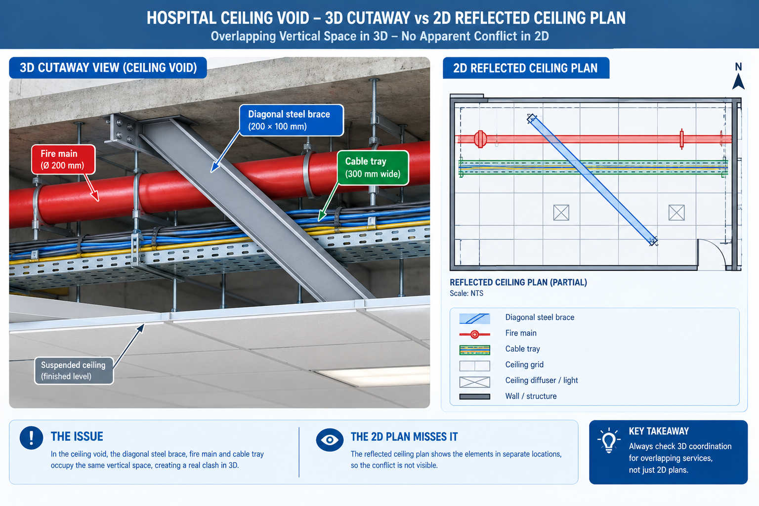
A 340-bed hospital project was six weeks from starting MEP rough-in on its fourth floor when the mechanical contractor’s foreman raised a question during a routine site walk: how was the fire suppression main, already fabricated and staged for installation, supposed to fit through the same 900mm ceiling void as the medical gas piping, the imaging suite’s cable tray, and the structural steel bracing installed two weeks earlier?
The 2D coordination drawings, produced by overlaying each trade’s reflected ceiling plan as flat, semi-transparent PDF layers, had shown no conflict. In three dimensions, the fire main, the cable tray, and a diagonal steel brace occupied the same 400mm of vertical space over an 18-metre run of corridor.
Quick answer: The conflict had existed since the structural bracing was added five months earlier, passing through three separate 2D drawing reviews because no single 2D overlay showed all three systems at once. This is the problem BIM clash detection exists to solve: three-dimensional conflicts that plan-view drawings, however carefully overlaid, cannot reliably reveal, because a 2D drawing collapses vertical position into a single flat view. Catching a conflict like this during design costs a few hours of model editing; catching it six weeks before fabricated pipe arrives on site costs nine days of schedule float and an emergency design change.
This article covers the five types of clashes a coordination process needs to catch, the measurable benefits of catching them before construction, the six-stage process that turns separate discipline models into a coordinated design, and a comparison of the tools used to run that process on real projects.
What BIM Clash Detection Actually Does
Clash detection is the automated process of testing the three-dimensional geometry of a federated Building Information Model, a shared model space bringing together individual discipline models from architecture, structure, mechanical, electrical, plumbing, and fire protection, to identify locations where elements from different systems conflict with each other or with a project rule. The output isn’t a design decision; it’s a list of specific, located conflicts, each tied to the exact elements involved and their model coordinates, that the coordination team then reviews, assigns, and resolves.
The distinction between clash detection and clash resolution matters because it defines what the software does versus what the process around it does. The software’s job is exhaustive and mechanical: test every element in one discipline’s model against every element in another’s, according to defined rules, and report every geometric overlap or rule violation, with no judgment about which conflicts matter most.
The coordination team’s job is everything after that: filtering out modelling artifacts that aren’t real conflicts, prioritising the ones that actually threaten schedule or budget, deciding which discipline moves, and confirming the fix worked. Treating the clash report as a finished deliverable rather than the start of a review process is one of the most common reasons coordination programmes underperform.
The Five Categories of Clashes a Coordination Process Should Test For
Relying only on hard-clash geometry testing misses the clearance, sequencing, and rule-based conflicts that cause just as much field disruption as a duct running through a beam.
Clash Type
Definition
Typical Example
Severity
Hard clash
Two physical elements occupy the same physical space
A structural beam passing through a ductwork run
Critical; cannot be built as drawn
Soft (clearance) clash
Elements don’t overlap but violate a required clearance or maintenance zone
A valve installed with less than code-required operating clearance
High; may install but creates an operational or compliance problem
Workflow (4D/sequencing) clash
No physical conflict, but construction sequence creates a scheduling or access conflict
A precast panel scheduled before the crane path is clear of scaffolding
Medium to high; causes schedule delay and resequencing
Non-collision clash (rule-based)
No overlap or clearance violation, but a business or design rule is violated
A duct routed through a designated clean room
Medium to high; life-safety and compliance rules often critical
Duplicate/redundant element clash
The same physical element modelled more than once by two disciplines
A structural engineer and architect both modelling the same slab edge
Low to medium; distorts quantities and coordination confidence
The Benefits of Clash Detection, Measured Where They Actually Show Up
The case for clash detection is easiest to make concretely: specific, measurable categories of cost and schedule risk shrink when conflicts are caught in the model instead of in the field.
Benefit
What It Solves
Where It Shows Up
Who Benefits Most
Reduced field rework
Physical conflicts discovered only when a crew tries to install the second system into occupied space
RFIs, change orders, demolition/re-installation cycles during rough-in
General contractors and MEP subcontractors carrying installation risk
Schedule certainty
Unplanned stoppages while a field conflict is redesigned and re-procured
Critical path activities in MEP and fire protection rough-in
Schedulers and owners with occupancy or lease-driven completion dates
Lower change order volume
Design conflicts caught only during construction, forcing an expensive change order
Owner change order logs
Owners and design teams carrying financial and reputational exposure
Earlier, cheaper design fixes
The same conflict is far cheaper to resolve as a model edit than a field fix
Design development and construction documentation phases
Design teams and owners managing a fixed design fee
Improved multi-trade coordination
2D overlay drawings don’t reliably reveal 3D conflicts in congested spaces
Coordination meetings across all disciplines
MEP coordinators and BIM managers running weekly meetings
Better as-built accuracy
Field-only fixes leave the model and as-built condition permanently out of sync
Facilities management handover
Facilities managers and owners operating the building long-term
Rework costs on uncoordinated projects are commonly cited at 5 to 10 percent of construction cost, and clash detection removes the large majority of the geometry-driven share of that figure. Model-based coordination is widely reported to substantially reduce coordination-related change orders compared with drawing-only coordination, consistent with the broader finding that the cost of correcting a coordination error rises by an order of magnitude at each stage it survives undetected.
What the Model-Based Process Would Have Caught
Had the hospital project run a federated clash test between the structural, mechanical, electrical, and fire protection models when the diagonal bracing was added, a hard clash between the brace and the fire main would have appeared automatically in that week’s clash report, five months before fabrication. The fix at that stage, adjusting the brace angle or rerouting a short section of the fire main, would have been a model edit costing a few hours of two disciplines’ time. The fix actually required, re-routing a fabricated fire main around an already-installed steel brace inside a congested ceiling void, consumed nine days of schedule float and required an emergency design change that delayed the floor’s inspection sign-off.
The Clash Detection Process: Six Stages From Federation to Closure
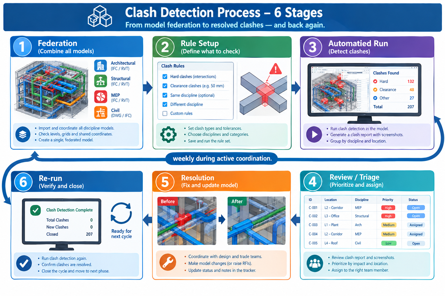
On any project of meaningful complexity, clash detection is a recurring cycle running throughout design development and continuing, at reduced frequency, through construction documentation and early construction.
Stage
What Happens
Common Pitfall
1. Model preparation and federation
Each discipline links its native model into a shared coordinate system inside a common platform
Mismatched origin points or level datums produce false clashes that waste review time
2. Clash test and rule set definition
The team defines which discipline pairs are tested, what clearance buffers apply, and which categories are excluded
Testing every discipline against every other with no buffers produces thousands of low-value soft clashes that bury critical hard clashes
3. Automated clash run
Software runs the defined tests and generates a report listing every detected conflict with location and severity
Running clashes only once at the end of design instead of on a recurring cycle lets conflicts accumulate undetected
4. Review, triage, and assignment
The team reviews the report together, confirms real conflicts versus false positives, and assigns ownership and priority
Reviewing clashes discipline-by-discipline in isolation lets each party defer resolution without a shared decision
5. Resolution and model update
The responsible discipline reroutes, resizes, or repositions the conflicting element and republishes the model
Resolving a clash locally without checking whether the fix creates a new conflict with a third, uninvolved discipline
6. Re-run and closure verification
The clash test is re-run to confirm the assigned clash is actually resolved and no new clash was introduced
Marking a clash closed based on a discipline’s report alone, without re-running the automated test
Why the Cadence of the Cycle Matters as Much as the Steps
A coordination process that runs these six stages once, at the end of design development, catches far fewer conflicts than the same process run weekly or biweekly throughout design, since every discipline is still actively changing their model, and a conflict introduced in week 10 won’t appear in a clash report generated in week 4. Mature coordination programmes typically run the full cycle weekly during the most active coordination phase, tapering to biweekly or on-demand once the clash count drops to a low, stable baseline.
The cadence also affects the coordination meeting itself. A team walking in with a clash report generated the same week discusses current, relevant conflicts. A team working from a month-old report is likely discussing conflicts one discipline has already partially resolved and others that no longer exist, wasting meeting time reconciling the report against the current model state before real coordination discussion can begin.
Clash Detection Tools: What Each One Is Actually Good At
No single tool covers every part of the process equally well. Most mature coordination programmes combine a geometric clash engine, a rule-based compliance checker, and increasingly a cloud-based issue tracker.
Tool
Primary Use Case
Typical Users
Notes
Autodesk Navisworks
Multi-discipline federation and automated clash detection
General contractors, MEP coordinators, BIM managers
Most widely used platform in construction; strong scheduling integration, steeper learning curve for rule-based setup
Solibri Model Checker
Rule-based model checking with strong code and standard compliance emphasis
Architects, code reviewers, owner QA teams
Particularly strong for non-collision and rule-based clashes; often used alongside Navisworks
BIM Collaborate (Autodesk Construction Cloud)
Cloud-based, continuous clash detection integrated with issue tracking
Distributed project teams needing real-time coordination
Removes manual federation, but requires all disciplines to publish to a shared cloud environment
BIMcollab
Cross-platform issue and clash management
Multi-vendor teams using different authoring tools
Uses BCF for cross-vendor issue exchange; typically manages clashes detected by another tool rather than detecting them itself
Trimble Tekla BIMsight/Connect
Federation and clash review for structural and precast-heavy projects
Structural engineers, precast/steel fabricators
Strong structural and fabrication-detail handling; less common as the primary MEP platform
Revit built-in interference check
Early, single-discipline or lightly federated checking during design development
Design teams performing preliminary self-checks
Useful first-pass check; not a substitute for a dedicated coordination platform
Choosing Between Desktop and Cloud-Based Coordination
The most consequential tool decision on most projects isn’t which specific software brand to use, but whether coordination runs on a desktop-federated model, where a BIM coordinator manually links each discipline’s exported file on a recurring cycle, or a cloud-based model, where each discipline publishes directly to a shared environment and clash detection runs automatically on every publish. Desktop federation gives more direct control over exactly which model versions are tested and is often preferred by small, co-located coordination teams. Cloud-based coordination reduces manual federation workload and gives near-real-time visibility, which tends to matter more with a large subcontractor pool or a geographically distributed design team.
Neither approach eliminates the need for review, triage, and resolution; a faster clash run only accelerates stage 3 of the six-stage cycle. Projects adopting cloud-based automatic clash detection without strengthening the review stage often end up with faster but not more effective coordination, more reports generated, same bottleneck at the human review stage.
Worked Examples
A commercial office tower ceiling void: A 32-storey office tower’s typical floor had a tightly constrained 600mm ceiling void carrying structural steel, HVAC ductwork, sprinkler mains, electrical bus duct, and data cable tray. Early coordination used 2D reflected ceiling plans reviewed independently by each trade, with the design team assuming the void depth was adequate based on a previous similar project.
The first federated clash test, run at roughly 60% model completion for mechanical and electrical, returned 340 hard clashes concentrated in the corridor zones outside the elevator core, where the largest primary ductwork, the fire sprinkler main, and the electrical bus duct all needed to cross the same limited ceiling void width at the same points. The clustering made clear that the 600mm void depth, adequate for a typical open office bay, wasn’t adequate where all major distribution systems converged near the core.
Rather than resolving 340 individual clashes one at a time, the coordination team used the clustering to identify the root design issue and raise it as a single decision: increase the void depth in that specific zone by 150mm, or reroute the primary ductwork through the adjacent open office bays instead. The team chose the reroute, implemented as a single change to the mechanical model. This resolved 312 of the 340 clashes in one model update, with the remaining 28 resolved individually in the next cycle. Because the pattern was caught at 60% model completion, the mechanical redesign was absorbed within the existing design schedule with no impact to the construction start date.
A precast parking structure column interface: A precast concrete parking structure had its column and beam connections modelled by the precast fabricator to a high level of detail, while the cast-in-place foundation and embedded electrical conduit were modelled separately by the structural and electrical engineers, on a coordination timeline running roughly two weeks behind the fabricator’s shop drawing schedule.
A clash test between the precast column base connection detail and the electrical conduit model found 14 hard clashes where embedded conduit for card-access control at ground-floor columns passed directly through the location reserved for precast column base plates and anchor bolts, a conflict invisible in either discipline’s drawings alone since the precast connection detail existed only in the fabricator’s shop model, not in the structural design model the electrical engineer had coordinated against.
Since the precast shop drawings were already in production and changing the anchor bolt pattern would have affected a connection type used at every ground-floor column, the team resolved the conflict by rerouting the conduit instead, adding a documented offset detail at each affected column. Resolving it as a single standard detail, rather than 14 separate site improvisations, meant the electrical contractor could issue one instruction covering every affected column, and the precast erection schedule proceeded without delay.
Frequently Asked Questions
At what stage of a project should clash detection start?
As soon as at least two disciplines have models with enough real geometry to test meaningfully, typically midway through schematic design or early design development, even with models still incomplete. Starting early catches large, structural-level conflicts (like the office tower ceiling void) while they’re still cheap to fix with a major routing decision, rather than waiting until construction documentation when the conflict can only be fixed by unpicking hundreds of already-detailed elements. Early clash detection produces more false positives from incomplete modelling, a reasonable cost for catching major conflicts while inexpensive to resolve.
Who is responsible for resolving a clash once it’s detected?
The clash report identifies the elements and disciplines involved, but resolution responsibility is typically assigned during review and triage based on project-specific coordination protocols, not automatically by the software. Common conventions: whichever discipline’s element is easier or cheaper to move (a duct is usually easier to reroute than a structural beam), whichever discipline routed later in the design sequence, or whichever the project’s coordination protocol designates as having priority in a given zone. These conventions should be agreed and documented before coordination begins, since disputes over whose model should change are a common source of resolution delay.
Does clash detection replace the need for a BIM coordinator or coordination meetings?
No. Clash detection software automates the geometric testing stage, but review, triage, assignment, and verification all require human judgment the software doesn’t perform. A BIM coordinator’s role shifts with mature tools from manually cross-checking drawings to managing the clash register, facilitating coordination discussion, and ensuring resolutions are actually verified by re-running the clash test, arguably a more valuable use of that role’s time, not one clash detection eliminates.
How many clashes is normal to find on a typical project?
Raw clash count varies enormously by project complexity, model maturity, and rule configuration, so it isn’t a meaningful benchmark alone. A more useful measure is the trend over time: a healthy programme shows open clash count rising as new disciplines’ models are added early in design, then declining steadily as resolution works through the backlog, converging toward a low, stable number by the time construction documents are issued. A flat or rising clash count through construction documentation signals the resolution stage isn’t keeping pace with detection.
Can clash detection be run without a full BIM model for every discipline?
Clash detection requires three-dimensional geometry to test, so a discipline still working in 2D drawings can’t be included in automated clash tests, limiting the programme’s coverage to disciplines that have modelled their scope in 3D. Many projects run a partial clash detection programme early, testing disciplines with adequate model maturity while others catch up, expanding the test matrix as more disciplines reach the required detail level. A project relying on 2D drawings for any major building system carries the same risk that produced the hospital corridor conflict, regardless of how well the 3D-modelled disciplines are coordinated.
Key Takeaways
The hospital corridor conflict existed in the design for five months before it was found, not because anyone reviewing the drawings was careless, but because the drawing format itself, separate 2D plan views, couldn’t show a three-way conflict between a diagonal brace, a duct, and a fire main occupying the same vertical space. This is the structural limitation clash detection exists to remove: three-dimensional conflicts require a three-dimensional test to be reliably found before they reach the field.
The office tower and precast parking structure examples show what that test looks like in practice: not a single pass/fail check, but a recurring cycle that surfaces conflicts early enough to fix as design decisions rather than field improvisations, and groups related conflicts so a team resolves a systemic issue once rather than fighting the same underlying conflict dozens of times. The software finds the conflicts; the process built around it, federation, rule definition, review, assignment, resolution, and verification, following the coordination protocols outlined in the National BIM Standard-United States, is what actually prevents them from reaching the job site.
Projects that treat clash detection as a checkbox run once before construction documents are issued get a fraction of its value. Projects that run it as a disciplined, recurring cycle throughout design, with a clear resolution protocol and a verified closure step, turn what’s otherwise an invisible risk, discovered only when a foreman looks up at the wrong moment, into a managed, tracked, and resolved part of the design process.
The engineer who has never encountered a scan-to-CAD conversion problem has not done enough scan-to-CAD conversion. The workflow looks straightforward in theory: scan the part, process the data, reconstruct the CAD model. In practice, the gap between those three steps contains ten categories of problems that each have their own technical root cause, their own detection method, and their own fix strategy. Understanding them transforms what feels like a frustrating collection of random failures into a systematic set of manageable engineering challenges.
This article exists because the previous article in this series, covering the complete reverse engineering workflow from scan to CAD model, documents what a successful workflow looks like. This article covers what happens when it does not go according to plan, which in practical engineering work is frequently. The challenges described here are not edge cases. They are the routine obstacles that every engineer executing scan-to-CAD conversion at production quality will encounter within their first ten projects.
Each challenge is covered with the specificity that makes it actionable: the underlying cause that explains why the problem occurs, the detection method that identifies it reliably (because many of these challenges are not immediately obvious), the primary fix strategy, and the alternative approaches when the primary fix is not sufficient or not applicable. The article closes with the legal and intellectual property considerations that every engineer doing competitive reverse engineering must understand, a topic that most technical content on this subject ignores entirely.
Challenge Overview: Root Cause, Detection, and Fix Strategy at a Glance
The following table maps all ten major challenge categories to their root cause, detection method, primary fix strategy, and severity classification. Use it as a quick reference when diagnosing a specific problem, and refer to the detailed section for each challenge for the full technical explanation.
Challenge
Root Cause
Detection Method
Primary Fix Strategy
Severity
Reflective and dark surface scan failure
Specular reflection or light absorption prevents pattern capture
Different materials reflect light differently within same scan
Boundary noise at material interfaces
Separate scan sessions per material, CT for embedded parts
High
CAD reconstruction quality vs mesh fidelity
Parametric reconstruction cannot capture all mesh detail
Deviation analysis of reconstructed CAD vs mesh
Hybrid approach: parametric for prismatic, NURBS for organic
Medium
Color and texture loss in geometry-only formats
STEP and IGES carry no color or texture data
Visual comparison, missing appearance data
Supplement with OBJ+MTL, VRML, or 3D PDF with texture
Low to Medium
The severity ratings reflect the impact on final CAD model quality if the challenge is not addressed: Very High challenges produce CAD models that are dimensionally incorrect and cannot be used for reproduction or manufacturing without causing failures. High challenges produce models with specific inaccurate regions. Medium challenges degrade model quality or workflow efficiency without necessarily invalidating the output.
Challenge 1: Reflective, Dark, and Transparent Surfaces
Surface optical properties are the most frequently encountered obstacle in structured light and laser line scanning, and they cause the most varied and unpredictable data quality problems. Three distinct surface conditions each create different failure modes: highly reflective surfaces, dark or absorptive surfaces, and transparent or translucent surfaces.
Reflective Surfaces: Specular Glare and Data Voids
Polished metals, chrome plating, mirror finishes, and wet surfaces create specular reflection: they reflect the scanner’s projected light pattern back at a specific angle rather than diffusing it across the field of view. When the camera is not positioned at the exact specular angle, it receives no light from that surface area and records no data. When it is near the specular angle, it receives saturated light that overwhelms the camera sensor, producing blown-out pixels with no useful fringe deformation information.
The characteristic signature of specular reflection in a point cloud is a pattern of voids surrounded by noisy data: the center of the reflection zone has no points (the camera received no return), surrounded by a fringe of noisy points (the camera received partially saturated return with corrupted fringe data). Attempting to fill these voids during mesh repair produces geometrically incorrect surfaces because the hole-filling algorithm has no scan data to work from in that region.
The primary fix is matte scanning spray: a temporary aerosol coating of white titanium dioxide or zinc oxide particles that provides a diffuse, lambertian-reflective surface for consistent light return from any camera angle. Applied correctly in 2 to 3 thin coats from 200 to 300mm distance, the coating is 5 to 15 microns thick and dries to a matte white finish that the scanner reads easily. For most mechanical engineering applications, this coating thickness is negligible relative to part tolerances. For precision surface measurements where the coating thickness matters, use the thinnest possible application and account for the coating thickness in your dimensional analysis.
A secondary approach is to adjust the scanner’s exposure settings to reduce sensitivity and capture less of the saturated reflection, or to reposition the scanner to avoid the specular angle for the most problematic surfaces. Most professional scanning systems allow per-scan exposure adjustment, and some support automatic multi-exposure capture (HDR scanning) that takes multiple exposures in the same position and combines the best data from each, effectively handling mixed reflectivity across a complex surface in a single capture.
Dark and Black Surfaces: Light Absorption
Dark surfaces, particularly matte black coatings, anodized aluminum, carbon fiber, and black rubber, absorb 80 to 95 percent of incident light. The scanner’s projected pattern reaches the surface but the reflected intensity is too low for the camera to detect reliable fringe deformation. The result is sparse, noisy point data rather than complete voids, because some light does return but the signal-to-noise ratio is too low for accurate position calculation.
The fix is the same matte scanning spray, which converts the dark surface to a diffuse white reflector. For parts where spray cannot be used (due to temperature sensitivity, chemical incompatibility, or requirement for an absolutely uncoated surface), alternative approaches include increasing the scanner’s projector intensity (if the system supports it), increasing exposure time, or switching to a laser line scanner rather than a structured light system, as laser line scanners are generally less sensitive to surface color than white-light structured light systems.
Transparent and Translucent Surfaces: Subsurface Scattering
Transparent materials (glass, clear acrylic, polycarbonate lenses) transmit the scanner’s light pattern rather than reflecting it, producing no data at all from the surface. Translucent materials (frosted plastic, skin, some composites) allow light to penetrate the surface and scatter within the material before returning, a phenomenon called subsurface scattering. This produces surface data that is systematically displaced from the true surface position by the scattering depth, typically 0.1 to 2 mm depending on material type and thickness.
Scanning spray converts transparent surfaces to opaque reflectors, resolving both problems. For parts where transparency is a functional property that must be preserved (optical components, light pipes, lenses), CT scanning is the only practical alternative for capturing the surface geometry without any surface preparation.
Surface Preparation Quick Reference Polished steel, chrome, aluminum mirror finish: 2 to 3 coats matte scanning spray. Anodized aluminum, black paint, carbon fiber: 2 to 3 coats matte scanning spray. Clear glass, polycarbonate, acrylic: 2 to 3 coats matte scanning spray (destroys transparency – use CT if optical function must be preserved). Rubber or silicone: Spray carefully – rubber can absorb spray solvent. Test on an inconspicuous area first. Alternative: use blue LED structured light rather than white LED for better rubber surface response.
Challenge 2: Inaccessible Geometry and Scan Shadows
Optical scanners, including structured light, laser line, and photogrammetry systems, share an absolute limitation: they can only capture surfaces they can see. Every feature that is occluded, recessed, or hidden behind another surface during scanning creates a scan shadow: a region of the point cloud with no data because no scan position had line-of-sight access to that surface.
Common examples include the interior of deep pockets, undercut features, the back face of a flange, the interior of a tube or bore, and the region under an overhang. In complex assemblies, adjacent components shadow each other, leaving interface surfaces without scan coverage.
Multi-Position Scanning to Minimize Shadows
The primary strategy for managing scan shadows is systematic multi-position scanning: planning the scan sequence so that every surface receives at least one scan position with acceptable line-of-sight access, even if that position is geometrically difficult to achieve. Before beginning any scan session on a complex part, walk around the part and identify every surface that will be difficult to access optically. Then plan the scanner positions, fixture orientations, and part repositioning steps needed to capture each of those surfaces.
For deep pockets and internal channels, scan from inside the pocket with the scanner tilted to the maximum possible angle. Most structured light systems capture data reliably at angles up to 45 degrees from the surface normal. Beyond this angle, the projected pattern becomes too foreshortened for accurate fringe deformation measurement, and data quality degrades rapidly. Laser line scanners generally have wider acceptance angles and can capture data at 60 to 70 degrees from normal in some configurations.
Industrial CT for Enclosed Internal Geometry
When optical scanning cannot capture required internal geometry regardless of the number of scan positions, industrial CT scanning is the definitive solution. CT sees through the material from all angles simultaneously, capturing internal surfaces, channels, wall thicknesses, and enclosed features that no optical scanner can reach. For hydraulic manifolds, castings with complex internal passages, sealed housings, and any assembly with interior surfaces that define function, CT is not an optional alternative to optical scanning. It is the only technology that captures the complete geometry.
The practical limitation is that CT requires access to a CT system (either in-house or as a service), it is slower than optical scanning, and it has part size constraints. For engineering teams that regularly reverse engineer complex internal geometry, CT scanning as a service from an industrial metrology provider is a practical and cost-effective solution for the cases where optical scanning cannot reach the needed surfaces.
Reconstructing Inaccessible Geometry by Inference
When CT scanning is not available and scan shadows cannot be eliminated through multi-position scanning, the engineer must reconstruct the unseen geometry by inference: using the surrounding scan data to determine what the hidden geometry must be, based on engineering knowledge, visual reference images, or measured cross-sections.
For features that follow predictable manufacturing patterns (a drilled and tapped hole that continues through to a visible back surface, a groove that follows a radius consistent with the cutter diameter visible in the surrounding material, a blind bore whose depth can be estimated from the visible part thickness minus a minimum wall thickness), reasoned reconstruction produces reliable results. For truly arbitrary hidden geometry with no inferential constraints, the CAD model must document the unknown region explicitly in its drawing annotations and inspection requirements.
Challenge 3: Part Deformation During Scanning
Part deformation during scanning is the most damaging challenge in the list because it is invisible in the scan data. The scanner captures the geometry of the part as it actually is during the scan, including any deformation caused by its own weight, by the fixture holding it, or by the thermal environment. The resulting CAD model accurately represents the deformed part, not the part’s true geometry, and the engineer may not discover the problem until a manufactured replacement using the CAD model does not fit correctly.
Gravity Sag in Large or Flexible Parts
Gravity sag is a common deformation mode for large parts, thin flexible sheets, rubber and elastomer components, and any part where the ratio of part mass to stiffness is high enough that measurable deflection occurs under self-weight. A long, thin aluminum extrusion lying horizontally will sag at its center. A rubber seal gasket deforms significantly under its own weight if unsupported. Even a relatively stiff steel bracket can show 50 to 200 microns of sag at its free end when cantilevered, which exceeds the accuracy of a high-quality structured light scan and would produce measurable dimensional error in the resulting CAD model.
The fix is fixture design: supporting the part in a way that replicates its functional configuration, or in a way that eliminates all gravity-induced deflection. For a part that is normally bolted flat to a surface, scan it in that bolted configuration with the mounting surface as the primary datum. For a part whose functional configuration cannot be determined, scan it from multiple orientations and compare the results to identify any gravity-dependent deformation in the data.
Fixture-Induced Stress
Fixtures that clamp or constrain a flexible part to hold it for scanning introduce their own deformation. The clamping force distorts the part geometry in the clamped region and can induce bending or twisting throughout the part. This is particularly problematic for thin-walled plastic parts, sheet metal, and rubber or silicone components. Fixture-induced deformation can be worse than unconstrained gravity sag if the fixture is not designed carefully.
Use the minimum clamping force required to hold the part stable during scanning. For very flexible parts, consider non-contact fixturing: a conformal nest made from foam or sand that supports the part across its full surface without applying point or line loads. For parts where any deformation is unacceptable, use gravity-independent measurement methods: CMM probing with the part in its functional installation configuration, or CT scanning where the part can be scanned while resting naturally without clamping.
Thermal Deformation
Temperature differences between the scan environment and the part’s functional operating temperature cause dimensional changes through thermal expansion. For a 200mm aluminum part (coefficient of thermal expansion approximately 23 microns per millimeter per degree Celsius), a 10 degree Celsius temperature difference between the scan environment and the nominal temperature produces 46 microns of dimensional change, which exceeds the measurement tolerance for precision features.
Ensure the part is at thermal equilibrium with the scan environment before scanning begins. For a part that has been transported from a cold or hot environment, allow 30 to 60 minutes of equilibration time before scanning. For precision work, record the ambient temperature during scanning and apply a thermal expansion correction to the scan data if the scanning temperature differs from the reference temperature (typically 20 degrees Celsius for engineering dimensional measurement per ISO 1 standard).
Deformation Risk Assessment Low risk: Rigid metal parts under 300mm, wall thickness over 5mm, scanned in ambient conditions. Medium risk: Parts over 500mm, thin-walled structures under 3mm, machined from stock (residual stress). High risk: Rubber/elastomer parts, flexible plastics, large sheet metal, assembled multi-material parts, parts transported from extreme temperatures. For High risk parts: design a dedicated scanning fixture, verify deformation by comparing scans in two different orientations, and consult a metrology engineer before committing the scan data to a CAD reconstruction.
Challenge 4: Distinguishing Wear and Damage from Original Geometry
This is the most engineering-intensive challenge in the entire scan-to-CAD conversion process because it cannot be resolved by any software tool or measurement technique alone. It requires engineering judgment informed by multiple lines of evidence, and getting it wrong produces a CAD model that faithfully reproduces a damaged part rather than the original design.
The specific problem: the scanned part has been in service and has accumulated geometric changes from in-service wear, impact damage, corrosion, plastic deformation, or fatigue-related distortion. The scan accurately captures the current state of the part, but the reverse engineering goal is typically to reproduce the original design geometry, not the worn state. The scan data alone cannot tell you what is original design geometry and what is accumulated damage.
Types of Geometric Change from Service Life
Abrasive wear produces gradual, smooth reduction in material at contact surfaces. It is typically most severe at sliding interfaces, sealing surfaces, and bearing surfaces. In a scan, worn surfaces appear as slight concavities or reduced thicknesses relative to the expected nominal geometry. Wear patterns are often asymmetric (one side wears faster than the other due to loading direction) and have a smooth, gradual boundary with unworn regions.
Impact damage produces local depressions, cracks, or material loss at specific locations from point loading events. These are typically more localized than wear and have sharper boundaries between damaged and undamaged regions. Impact damage can produce significant local deformations: a 20mm dent in a steel plate from a dropped tool can represent 2 to 5mm of surface displacement.
Corrosion produces surface texture changes and material loss at chemically active surfaces. Early-stage corrosion produces a roughening of the surface texture that increases scan noise without significant dimensional change. Advanced corrosion produces measurable material loss and surface pitting that significantly corrupts the scan data in affected regions.
Plastic deformation from overloading produces permanent geometric change throughout the affected region. Unlike wear (which only removes material from contact surfaces) or impact damage (which is localized), plastic deformation can alter the geometry of large regions of the part in ways that are difficult to identify from the scan alone without reference to the original design dimensions.
Strategies for Identifying Wear and Damage
Use multiple evidence sources in combination to identify which geometric deviations are wear and which are original design features:
Compare to surviving unworn regions: Most worn parts have some surfaces that were not in contact with anything during service and remain at or near the original geometry. Comparing the worn surfaces to these reference regions establishes what the original dimensions likely were.
Statistical analysis of the point cloud: Wear and damage produce localized outlier deviations from the general surface geometry. Fitting a geometric primitive to the entire surface and examining the residual deviation distribution identifies regions where the deviation is anomalously large, indicating either damage or an intentional geometric feature. Large, localized positive deviations suggest material buildup or deformation. Large, localized negative deviations suggest wear or removal.
Multiple part comparison: If more than one example of the same part is available, scanning multiple examples and comparing them isolates genuine design geometry (consistent across all parts) from wear and damage (variable between parts depending on service history).
Physical reference standards: Assembly drawings, inspection sheets, or supplier part numbers from the original program may establish nominal dimensions against which the scan can be compared, identifying the magnitude and location of all deviations from nominal.
Manufacturing process inference: An engineer familiar with the manufacturing process for the part type can identify which surfaces would have been machined to a precise nominal and which would have been cast or formed with greater variation. Machined surfaces in an unworn state should have scan residuals close to the scanner’s measurement uncertainty. Larger residuals on machined surfaces indicate either wear or damage.
Challenge 5: The Symmetry Assumption Trap
The symmetry assumption trap is a specific error pattern that is extremely common among engineers who are new to scan-to-CAD conversion and surprisingly persistent among experienced ones. It occurs when an engineer, modeling a part that appears symmetric from visual inspection, applies symmetry in the CAD reconstruction without verifying from the scan data whether the part is actually symmetric within measurement precision. The result is a CAD model that is more symmetric than the physical part, which can cause fit errors in asymmetric assembly interfaces and incorrect mass properties.
Most manufactured parts that are nominally symmetric are not perfectly symmetric in their as-built state. Casting, forging, and injection molding processes all introduce manufacturing variation that is rarely perfectly symmetric. In-service loading can induce asymmetric wear or deformation. And some parts that appear symmetric actually have subtle intentional asymmetry that serves a functional purpose, such as a poka-yoke feature that prevents incorrect installation.
Detecting Asymmetry in Scan Data
The detection method is a mirror comparison analysis: reflect the scan data about the presumed plane of symmetry and compute the deviation between the original data and its mirror image. If the part is truly symmetric within the measurement uncertainty of the scanner, the deviation between original and mirror should be uniformly distributed at or below the scanner’s noise level. If specific regions show systematic deviation above the noise level, those regions are genuinely asymmetric.
Most professional scan processing software (Geomagic, PolyWorks, ZEISS Inspect) includes symmetry analysis tools that perform this comparison automatically and display the results as a color map. This analysis should be performed before any symmetry is applied in the CAD reconstruction, and its results should be documented in the project record.
The Right Response to Detected Asymmetry
When the symmetry analysis reveals asymmetry, the engineer must determine whether it represents manufacturing variation that should be idealized away or intentional design asymmetry that must be preserved. Manufacturing variation is typically random in distribution and magnitude, with no consistent directionality. Intentional design asymmetry is typically consistent across multiple examples of the same part and associated with a functional interface or assembly constraint.
For manufacturing variation: apply symmetry in the CAD model and document the decision with the measured asymmetry magnitude. For intentional asymmetry: model the asymmetric geometry explicitly and investigate whether the asymmetry is a poka-yoke feature, a balancing provision, or a functionally significant geometric difference that affects part performance or assembly.
Challenge 6: Thread and Fine Feature Reconstruction
Thread reconstruction from scan data is a universally acknowledged limitation of optical scanning, and it is one area where the standard workflow must be supplemented by a different measurement approach. No current optical 3D scanner reliably captures thread geometry with enough accuracy for thread profile reconstruction. Thread pitches for common metric threads range from 0.35 mm for M2 to 3 mm for M36. The helix angle, flank angle, root radius, and crest geometry of a standard thread are all at a scale that is either below the resolution of most industrial scanners or creates such extreme surface angle variation that the scan data is too noisy to extract meaningful thread geometry.
Why Threads Cannot Be Scanned Reliably
The fundamental problem is geometry, not scanner quality. Thread flanks on a metric thread have a 60-degree included angle, meaning the thread faces are inclined at 30 degrees from the axis. At the root of the thread, the scanner must capture a surface that is deeply recessed between two flanks, at an angle that may exceed the scanner’s angular acceptance. Even when data is captured in the thread region, the thread root and crest radii are typically below the spatial resolution of most structured light systems (typically 0.1 to 0.3 mm point spacing for medium parts). The resulting point cloud in the threaded region is too sparse and noisy to extract reliable thread profile data.
The Hybrid Measurement Approach
The correct approach for threaded features is hybrid measurement: scan the part optically to capture all non-threaded geometry, and measure all threaded features separately using a method appropriate for thread metrology: optical comparator, thread gauge, thread micrometer, or CMM probing with a thread-pitch measuring strategy.
The optical scan provides the position of the threaded bore’s axis (captured from the cylindrical bore surface surrounding the thread), the bore diameter (from the cylinder fit to the major diameter region), and the depth of blind holes. CMM measurement or gauge measurement provides the thread specification: pitch, thread form (metric, UNC, UNF, ACME, etc.), tolerance class, and depth of engagement. The CAD reconstruction combines both sources: the scan-derived position and the gauge-derived thread specification.
Fine Features Below Scanner Resolution
Beyond threads, any geometric feature whose characteristic dimension is smaller than the scanner’s point spacing is potentially affected by resolution-limited reconstruction. Knurling, fine surface textures, small radii (under 0.2 mm), sharp edges (the scanner captures a blend radius that does not exist in the physical part), and fine engraved markings are all below the resolution of most industrial scanners.
For sharp edges and small radii: document the expected nominal value (based on manufacturing process knowledge or reference drawings) and use this nominal value in the CAD model rather than trying to extract it from the scan. A milled part has sharp internal corner radii equal to the end mill radius used. A cast part has minimum radii defined by the mold tool design. These values are more reliably determined from manufacturing process knowledge than from scan data.
Challenge 7: Data Volume and Processing Performance
Modern structured light scanners produce point clouds of 5 to 50 million points per scan position, and complex parts requiring 20 to 40 scan positions produce raw datasets of 100 million to 2 billion points. Processing, registering, and reconstructing CAD geometry from datasets at this scale places substantial demands on workstation hardware, and underpowered workstations are one of the most common practical bottlenecks in scan-to-CAD workflows, causing software crashes, multi-hour processing times for operations that should take minutes, and workflow interruptions that disrupt the engineer’s focus.
The Computational Bottleneck Explained
Point cloud processing operations, particularly ICP registration (which iteratively compares millions of point pairs), mesh generation (which builds topological relationships across hundreds of millions of points), and NURBS surface fitting (which involves large matrix operations), are computationally intensive in specific ways that determine which workstation specifications are most impactful.
RAM is the primary constraint for large dataset operations: a 500-million-point dataset requires 6 to 10 GB of RAM just to hold the point coordinates in memory before any processing begins, and processing operations create temporary copies and work arrays that multiply the memory requirement by 3 to 5 times. Geomagic Design X recommends a minimum of 32 GB RAM for complex scan projects. 64 GB is strongly preferred for large industrial parts. 128 GB is appropriate for very large assemblies or complex organic forms with dense scan data.
CPU performance matters for single-threaded operations like ICP refinement and geometry healing, which benefit from high per-core clock speeds. GPU acceleration is increasingly used by modern scan processing software for mesh generation and surface fitting. Fast NVMe SSD storage is essential because scan datasets routinely exceed the size that fits in RAM and must be streamed from disk during processing. A mechanical hard drive accessing 100 GB of scan data during processing creates wait times that can multiply the total workflow time by 5 to 10 times compared to NVMe storage at the same dataset size.
Practical Strategies for Managing Data Volume
Uniform downsampling before any processing: Reduce the point cloud to the minimum density that preserves all relevant geometric detail (typically 0.05 to 0.2mm point spacing for industrial parts). This reduction alone cuts processing time by 80 to 95 percent for most operations.
Region-of-interest processing: Process the scan in sections rather than all at once. Work on each sub-region at the resolution it requires, combining the final processed regions at a later stage.
64-bit operating system and application: Verify that the scan processing software is running in 64-bit mode (not 32-bit compatibility mode), which allows access to more than 4 GB of RAM per process.
Temporary file location: Configure the scan software’s scratch/temporary file directory to point to the fastest available storage (NVMe SSD, not a network drive or mechanical HDD).
Background process management: Close all non-essential applications during intensive scan processing operations to maximize available RAM and CPU bandwidth for the scan software.
Minimum Workstation Specification for Scan-to-CAD Work WORKSTATION REQUIREMENTS FOR SCAN-TO-CAD CONVERSION:
SMALL PARTS (under 200mm, single setup, < 50M points): CPU: Intel i7 or AMD Ryzen 7, 8+ cores, 3.5GHz+ RAM: 32 GB DDR4 (3200MHz recommended) GPU: NVIDIA Quadro/RTX 4000+ or AMD Radeon Pro equivalent Storage: 500 GB NVMe SSD (OS+Software) + 1TB NVMe SSD (project data) Display: 2560x1440 IPS or better (color accuracy matters for deviation maps)
LARGE ASSEMBLIES (600mm+, complex multi-material, >500M points): CPU: Dual-socket Xeon or AMD EPYC, 32+ cores total RAM: 128 GB minimum - 256 GB preferred GPU: NVIDIA RTX A6000 or better (VRAM >= 24 GB) Storage: RAID-0 NVMe array for scratch data, minimum 4 TB Note: Consider cloud processing for extreme dataset sizes
Challenge 8: Multi-Material Scan Artifacts
Parts made from multiple materials with different optical properties create a specific and often overlooked scan challenge: the scanner is calibrated and optimized for one set of optical conditions, but the part presents multiple different conditions simultaneously. At the boundary between materials with different reflectivity or color, the scanner produces noisy or incorrect data in a zone that extends 1 to 5 millimeters on either side of the material interface.
A metal housing with a rubber gasket face is a classic example. The metal face may require normal exposure settings for the structured light projector. The rubber gasket may require higher exposure and a different angle because it is darker and absorbs more light. At the gasket-to-metal interface, the scan data transitions between these two conditions and produces a noisy boundary zone. The CAD reconstructed from this data shows an inaccurate representation of the interface geometry, which may be the most functionally critical surface in the whole part.
Material Boundary Management Strategies
Strategy 1: Separate scan sessions per material region. Scan the metal faces first with the optimal settings for metal, and the rubber faces in a separate session with adjusted settings. The two sessions are registered together in the same coordinate system using the common coded targets that remain in place throughout both sessions. This approach produces optimal data quality for each material region but requires careful planning to ensure that every surface region belongs clearly to one session or the other, and that enough overlap exists at the boundaries for registration.
Strategy 2: HDR multi-exposure scanning. Some advanced structured light systems support High Dynamic Range scanning, where multiple exposures are taken at each scan position and merged to produce a single point cloud that combines the best data from each exposure level. This effectively handles mixed reflectivity within a single scan session and is the most convenient solution when the equipment supports it.
Strategy 3: Industrial CT for embedded and multi-material assemblies. When the multi-material interface is critical for dimensional accuracy and optical scanning consistently produces poor results at that interface, CT scanning provides accurate geometry for both materials simultaneously, independent of their optical properties. The CT image segments each material based on its X-ray attenuation, which varies by density and atomic composition, providing clean boundaries between material regions even when their optical properties are similar.
Overmolded Parts: A Specific Multi-Material Challenge
Overmolded components, where a soft material is molded over a rigid substrate, present a particular challenge because the soft overmold material deforms differently from the rigid substrate during scanning. If the part is handled or fixtured, the soft overmold deforms at the handling points. If it is scanned without support, gravity causes the overmold to sag. And at the interface between the rigid substrate and the soft overmold, the scan data captures the outer surface of the overmold but provides no information about the substrate geometry beneath it. For overmolded parts where the substrate geometry is functionally critical, CT scanning is the only method that captures both surfaces reliably
Challenge 9: Balancing CAD Model Quality Against Mesh Fidelity
There is an inherent tension in scan-to-CAD conversion between two competing quality goals: geometric fidelity to the scan data and CAD model quality and usability. The mesh produced from the scan data captures every surface irregularity in the physical part: manufacturing variation, surface roughness, minor damage, and scan noise are all present in the mesh as genuine geometric features. A CAD model that precisely reproduces every detail of the mesh is geometrically accurate to the scan but may be extremely difficult to use for design modification, drawing generation, or FEA because of its complexity and lack of parametric structure.
The engineer must make deliberate decisions about how much mesh detail to preserve in the CAD model and how much to idealize. These decisions should be documented so that anyone reviewing the CAD model can understand what level of idealization was applied and what the underlying scan data showed.
The Four Levels of Mesh Detail in CAD Reconstruction
Level 1: Exact mesh representation – The mesh itself is the CAD output. No parametric reconstruction is performed. The mesh is cleaned, repaired, and exported as STL, OBJ, or similar format. Appropriate when the output is for 3D printing, visualization, or simulation where mesh input is accepted and parametric CAD is not required.
Level 2: NURBS surface fit to mesh – NURBS surfaces are fitted to the mesh regions, capturing the general shape including manufacturing variation. The resulting surfaces are smooth but not perfectly prismatic. Appropriate for organic forms and consumer product surfaces where the general manufactured shape is what needs to be captured.
Level 3: Fitted primitives with as-built dimensions – Geometric primitives (planes, cylinders, spheres) are fitted to the mesh and the as-built dimensions are extracted. The CAD model uses these as-built values directly as driving dimensions. Appropriate for exact reproduction where every dimensional deviation from nominal is intentional and must be preserved.
Level 4: Idealized parametric reconstruction – Geometric primitives are fitted to the mesh, nominal dimensions are inferred by rounding to standard values, and the CAD model is built as a fully parametric part with clean feature tree, named parameters, and nominal dimensions. Appropriate for design intent recovery and downstream modification.
The choice between these levels should be made explicitly at the beginning of the project based on the engineering intent defined in the previous article. Defaulting to Level 4 for all projects adds unnecessary modeling time. Defaulting to Level 1 produces output that is often unusable for engineering purposes. Matching the level to the application makes the project efficient and the output fit for purpose.
Challenge 10: Legal and Intellectual Property Considerations
This challenge is categorically different from the nine technical challenges above. It is not a data quality problem or a workflow efficiency problem. It is a legal risk that applies specifically to competitive reverse engineering: the process of scanning and recreating a product manufactured by another organization for the purpose of understanding, competing with, or reproducing that product.
Most scan-to-CAD content for engineers treats this topic as outside scope. That is a significant disservice, because engineers executing competitive reverse engineering programs without understanding the applicable legal framework are exposing their organizations to significant liability. The legal landscape is complex, jurisdiction-dependent, and evolving, and this article is not a substitute for qualified legal advice. But the framework below provides the starting orientation that every engineer doing competitive reverse engineering needs.
What Is and Is Not Protected by Intellectual Property Law
Patents protect functional inventions for a limited term (typically 20 years from filing). A patented mechanism, assembly method, or process cannot be reproduced without a license regardless of how the reproduction is achieved, including by scanning the patented product. Before conducting reverse engineering of a competitor’s product, check whether the functional aspects of interest are patented in the jurisdictions where the reproduction will be manufactured and sold.
Trade dress protects the distinctive visual appearance of a product or its packaging. If the exterior appearance of a product has been registered as trade dress, creating a CAD model that reproduces that appearance and using it to manufacture a competing product may infringe the trade dress even if the functional geometry is not patented.
Copyrights do not typically protect functional three-dimensional objects (as opposed to artistic or sculptural works), but software embedded in a product, digital design files obtained directly from a manufacturer, and decorative or artistic surface features may be copyright-protected.
Trade secrets protect confidential information that has economic value from its secrecy. If information about a product was obtained through a confidential relationship (such as a supplier agreement that included non-disclosure obligations), using that information in a reverse engineering program may breach the confidentiality agreement regardless of whether the information itself is patented.
The Legitimate Uses of Competitive Reverse Engineering
In most jurisdictions, reverse engineering a legally purchased product for interoperability, compatibility, or research purposes is a legally protected activity, provided the product was purchased lawfully and no contractual restriction on analysis was agreed to at purchase. Manufacturing and selling a competing product that reproduces patented functionality is not protected. Manufacturing and selling a competing product that provides the same function through a non-infringing design (informed by understanding the competitor’s approach through reverse engineering) is generally protected.
The practical implication for engineering teams is: document the purpose of the reverse engineering program clearly at its outset. Engineering understanding of a competitor’s design approach for the purpose of designing a non-infringing alternative is legally very different from engineering a direct copy. If the purpose is not clearly documented, a court may draw unfavorable inferences about intent from the existence of scan data and CAD models of a competitor’s product.
Legal Caution This section provides only a general orientation to intellectual property considerations in reverse engineering. It does not constitute legal advice. Before committing to any competitive reverse engineering program that will result in a commercial product, consult qualified intellectual property counsel in the relevant jurisdictions. The legal framework varies significantly between countries (particularly between the US, EU, and Asian jurisdictions), between industries, and based on the specific facts of each situation.
Frequently Asked Questions
Q: Why do I get holes and voids in my 3D scan data?
Holes and voids in 3D scan data have three main causes: line-of-sight limitations (the scanner cannot see surfaces hidden behind other geometry), surface optical properties (reflective surfaces create specular glare voids, dark surfaces create sparse data, transparent surfaces produce no data), and scanner standoff angle violations (data captured at too shallow an angle to the surface produces noise or voids). The fix depends on the cause: add scan positions to reach hidden surfaces, apply matte scanning spray for optical surface issues, or use industrial CT scanning for enclosed internal features that optical scanners cannot reach.
Q: How do I scan reflective metal parts without getting glare artifacts?
Apply a matte anti-glare scanning spray (titanium dioxide or zinc oxide aerosol) to the reflective surface in 2 to 3 thin coats from 200 to 300mm distance. The 5 to 15 micron coating provides a diffuse, lambertian-reflective surface that the structured light scanner can capture accurately from any angle. The coating is temporary and can be washed off after scanning with water or a mild solvent. For highly polished precision surfaces where coating thickness matters, apply the thinnest possible coat and account for the coating thickness (typically 5 to 10 microns) in your dimensional analysis. Alternative approaches include HDR multi-exposure scanning or adjusting the scanner angle to avoid the specular reflection zone.
Q: Can I accurately reconstruct thread dimensions from a 3D scan?
No, optical 3D scanning cannot reliably capture thread geometry at the accuracy required for thread specification reconstruction. Thread pitches for common fasteners range from 0.35mm to 3mm, and the thread root radius and flank geometry are at a scale below the resolution of most industrial scanners. The correct approach is hybrid measurement: scan the part optically to capture the bore position and major diameter, then measure the thread specification separately using a thread gauge, optical comparator, or CMM probing. Combine both data sources in the CAD reconstruction: scan-derived position and gauge-derived thread specification.
Q: How do I tell whether a dimensional deviation in my scan is wear or original design geometry?
Compare the deviation against multiple evidence sources: surviving unworn surfaces on the same part (which should remain near the original design geometry), statistical analysis of the point cloud to identify systematic vs random deviations (wear is typically smooth and directional, design features are consistent and bounded), comparison across multiple examples of the same part if available (wear varies with service history, design features are consistent), and manufacturing process inference (machined surfaces should have scan residuals near the scanner noise level if unworn). When in doubt, document the uncertainty explicitly and flag the affected dimensions for verification before any manufacturing commitment.
Q: What workstation specifications do I need for scan-to-CAD work?
For medium-complexity industrial parts producing 50 to 500 million points: 64 GB RAM (minimum, 128 GB preferred), Intel i9 or AMD Threadripper CPU with 16+ cores, NVIDIA RTX 4080 or better GPU with at least 16 GB VRAM, and NVMe SSD storage for both the operating system and project data. RAM is the primary bottleneck: scan processing creates multiple temporary copies of large datasets simultaneously. NVMe SSD storage is the second most impactful specification because large datasets must be streamed from disk during processing. A mechanical hard drive accessing large scan data can multiply total processing time by 5 to 10 compared to NVMe storage.
Q: Is reverse engineering a competitor’s product legal?
It depends on the jurisdiction and the specific purpose. In most jurisdictions, reverse engineering a legally purchased product for purposes of interoperability, research, or designing a non-infringing alternative is a legally protected activity. However, reproducing patented functionality, infringing registered trade dress, or using information obtained under a confidentiality obligation can create significant legal liability regardless of how the reverse engineering was conducted. The specific legal framework varies between countries and industries. Before commencing any competitive reverse engineering program intended to result in a commercial product, obtain qualified legal advice from intellectual property counsel in the relevant jurisdictions. Document the purpose of the program clearly at its outset.
Q: Why does my CAD model not match the scan data in the final deviation analysis?
Large deviation analysis discrepancies have several common causes: incorrect primitive fitting (the plane or cylinder fit did not capture the true geometry of that region), design intent rounding to nominal that moved a dimension outside the measurement uncertainty range, part deformation during scanning that was not detected and corrected, wear or damage on the scanned part that was inadvertently reproduced in the CAD model, or a registration error in the point cloud that introduced a systematic misalignment. The deviation analysis color map identifies exactly where the CAD model deviates from the scan. Return to the reconstruction for each high-deviation region and re-examine the fitting or modeling decision that produced the deviation.
Conclusion:
The ten challenges covered in this article account for the overwhelming majority of the problems that engineers encounter in scan-to-CAD conversion workflows. None of them are random or unpredictable. Each has a specific root cause that explains why it occurs, a specific detection method that identifies it before it corrupts the final output, and a specific fix strategy that resolves it when it is detected.
The pattern across all ten challenges is consistent: problems that are detected early in the workflow are solved cheaply. Problems that reach the CAD reconstruction stage, or worse, the deviation analysis stage, are solved expensively. Surface preparation before scanning is ten minutes. Discovering missing scan data after the scanner has been returned to its case and the part has been cleaned is a rescan request. Detecting asymmetry before applying symmetry in CAD is a five-minute analysis. Discovering the asymmetry error after completing the parametric reconstruction is an hours-long rework.
Build the pre-scan checklist, the intermediate quality checks, and the final deviation analysis into every scan-to-CAD project as non-negotiable workflow steps. The engineers who execute scan-to-CAD conversion at the highest reliability are not the ones who never encounter these challenges. They are the ones who detect and address each challenge at the earliest possible workflow stage, before it becomes a project-level problem.
Build your complete scan-to-CAD knowledge with our guide to the full reverse engineering workflow, CAD data translation problems, parametric modeling best practices, and multi-body modeling techniques.
3D modeling in CAD is the technical discipline at the heart of modern engineering and design. Every car that drives, every aircraft that flies, every medical device that saves a life, and every building that stands was first created as a precise 3D digital model before a single physical component was manufactured or a foundation was dug. The 3D CAD model is where engineering creativity becomes engineering reality.
Yet despite its central importance, 3D modelling in CAD is one of the least well-explained topics in engineering education. Most tutorials cover how to use a specific tool’s commands. Very few explain what is actually happening mathematically when you extrude a profile, why parametric modelling works the way it does, when surface modelling is the right approach versus solid modelling, how to plan a model structure so it remains editable under future design changes, or how to validate a 3D model before releasing it for manufacture.
This pillar guide closes all of those gaps. It covers 3D modelling in CAD from first principles through to advanced professional practice: the five modelling paradigms and their underlying mathematics, the complete 3D modelling workflow from concept to verified model, assembly modelling and large assembly management, advanced techniques including topology optimisation and generative design, industry-specific workflows across six engineering disciplines, model quality and validation, the best tools for each type of 3D modelling work, the integration of 3D models with simulation and manufacturing, and the AI-driven changes reshaping the discipline in 2026.
Quick Definition: 3D modeling in CAD is the process of creating a complete three-dimensional digital representation of a physical object or system using computer-aided design software. The resulting 3D model defines the object’s geometry with engineering precision, it can be measured, analysed, modified, used to generate manufacturing instructions, and used as the basis for structural or fluid dynamic simulation. It is the primary method by which engineering designs are created, communicated, and verified in the modern engineering profession.
What Is 3D Modeling in CAD? Foundations and Purpose
3D modeling in CAD is the creation of a mathematically defined three-dimensional digital object within a computer-aided design software environment. Unlike a 2D drawing, which represents an object through multiple flat views and relies on the reader to reconstruct the 3D form mentally, a 3D CAD model is a complete, unambiguous representation of the object that exists in three-dimensional coordinate space with exact geometric definition.
The fundamental difference between a 3D CAD model and a 3D model created in general-purpose software (such as Blender or 3D Studio Max for visual effects) is engineering precision. A 3D CAD model is defined in real-world measurement units (millimetres, inches, metres) with exact dimensional values. Every face, edge, and vertex has a precise mathematical location in the coordinate system. The model can be interrogated to return mass, volume, centre of gravity, moments of inertia, and surface area, properties that are essential for engineering analysis.
Why 3D Modeling Changed Engineering Practice
Before 3D CAD modeling became mainstream in the 1990s, engineers designed products entirely in 2D: producing multiple orthographic views of each component and mentally synthesising them into an understanding of the 3D form. This process was slow, error-prone (particularly for complex geometry), and made it extremely difficult to detect interference between components in an assembly before physical prototypes were built.
The introduction of parametric 3D solid modelling, pioneered by Pro/ENGINEER in 1987 and brought to the mass market by SolidWorks in 1995, transformed this workflow. Engineers could now design in 3D directly, visualise the product from any angle, detect clashes automatically, generate all 2D views simultaneously from the single 3D master model, and hand the model directly to simulation software for analysis and to CAM software for manufacturing programming.
According to Aberdeen Group research, companies that use 3D CAD modeling reduce time-to-market by an average of 50 percent compared to 2D design workflows, reduce manufacturing errors by 65 percent, and reduce the cost of design changes by up to 90 percent when changes are made in the 3D model rather than after physical production.
Benefit of 3D CAD Modeling
Specific Advantage
Industry Impact
Spatial visualisation
Design can be viewed from any angle, rotated, sectioned, and animated
Dramatically reduces interpretation errors between designers and manufacturers
Automatic 2D drawing generation
Orthographic views, sections, and details generated automatically from the 3D model
Eliminates the manual drawing board workflow; drawing updates automatically when model changes
Interference and clash detection
Software automatically identifies where two components physically overlap in an assembly
Prevents manufacturing of components that cannot be assembled, historically discovered only at first physical build
Mass properties calculation
Weight, centre of gravity, moments of inertia calculated directly from the solid model geometry
Enables structural analysis, balance calculations, and manufacturing cost estimation without physical prototypes
Simulation input
3D geometry used directly as input for FEA stress analysis, CFD, and thermal simulation
Reduces physical prototype testing cycles; finds structural or thermal issues before manufacture
Manufacturing programming
CNC toolpaths generated directly from the 3D model surface geometry
Eliminates manual programming for complex 3D machined surfaces; reduces errors in manufacturing instructions
Product visualisation and rendering
Photorealistic images and animations produced before physical product exists
Enables client approval and marketing before tooling investment
The Five 3D Modeling Paradigms Explained
3D modeling in CAD is not a single methodology. It encompasses five distinct paradigms, each based on different mathematical representations of geometry and each suited to different design tasks. Understanding all five, and knowing when to apply each, is what separates a proficient 3D modeller from an expert one.
Paradigm
Mathematical Foundation
Primary Strength
Primary Limitation
Best Application
Solid Modeling (B-rep)
Boundary Representation: solid defined by closed set of faces, edges, vertices
Physically complete, mass properties calculable, FEA-ready, Boolean operations
Triangulated or quadrilateral polygon mesh approximating surface
Handles complex organic shapes, fast for visualisation, 3D printing compatible
Not dimensionally precise; not manufacturing-ready without conversion
3D printing, visual rendering, scan-to-CAD, game assets, organic forms
Paradigm 1: Solid Modeling (B-rep)
Solid modeling using Boundary Representation (B-rep) is the foundational paradigm of engineering CAD. A B-rep solid is a complete, closed, watertight volumetric object defined by the mathematical surfaces that bound it, faces, edges (where faces meet), and vertices (where edges meet). The geometric kernel (Parasolid or ACIS in most commercial tools) maintains the topological relationships between all these elements to ensure the model is always a valid, manifold solid.
What B-rep Solid Modeling Enables
The completeness of the B-rep representation, the fact that the solid is fully enclosed with no gaps or self-intersections, is what enables mass properties calculation (the kernel can integrate over the enclosed volume to compute mass, centre of gravity, and inertia tensor), Boolean operations (precisely cutting one solid from another using the mathematical intersection of their boundary surfaces), and automatic generation of 2D section views (cutting the solid with a plane to produce a precise cross-sectional profile).
Boolean Operations in Solid Modeling
The three fundamental Boolean operations in solid modeling are mathematically equivalent to set operations applied to the volumetric regions bounded by the solids:
Union (A U B): Creates a new solid that encloses all points inside either solid A or solid B. Used to combine separate solid features into one body.
Intersection (A n B): Creates a new solid that encloses only points inside both solid A and solid B simultaneously. Used to find the overlapping volume of two solids.
Difference (A – B): Creates a new solid that encloses points inside solid A but not inside solid B. This is the mathematical foundation of the SUBTRACT command, cutting a hole, pocket, or channel.
Engineering Context: When an engineer subtracts a cylinder from a box to create a hole, the CAD software is computing the set difference A – B between the B-rep solid of the box and the B-rep solid of the cylinder, then rebuilding the resulting boundary surface topology. This is why the hole has perfectly cylindrical interior walls that are tangent to the box faces, the result is geometrically exact, not an approximation.
Paradigm 2: Parametric Feature-Based Modeling
Parametric feature-based modeling extends B-rep solid modeling by adding two critical layers: a feature history that records the sequence of operations used to build the model, and a constraint system that maintains the geometric relationships between elements. Together, these layers encode the engineer’s design intent, the rules that govern how the model should change when parameters are modified.
The Feature History Tree
The feature tree (model tree or design tree) is a chronological record of every operation applied to the model. It might read: Base Extrusion > Fillet > Through Hole > Hole Pattern > Chamfer > Thread. Each entry in the feature tree is a parametric feature, an operation defined not just by the geometry it produces but by the parameters that govern it (extrusion depth, fillet radius, hole diameter, pattern count and spacing).
When a parameter is changed, for example, the extrusion depth is increased from 50mm to 75mm, the CAD system rebuilds the model from that feature downward in the feature tree. The fillet, hole, pattern, chamfer, and thread all update automatically, because they are defined relative to the base extrusion geometry that has just changed. This automatic propagation is design intent in action: the engineer specified that the fillet is on the top edge of the base extrusion, so wherever the top edge goes, the fillet follows.
Sketches and 2D Profiles as Parametric Foundations
Most parametric features begin with a 2D sketch, a constrained 2D profile drawn on a reference plane or an existing face. Sketches contain geometric constraints (horizontal, vertical, coincident, tangent, perpendicular) and dimensional constraints (length = 100mm, angle = 45 degrees). When the sketch is fully constrained, it has no remaining degrees of freedom: every point is exactly located.
The rule for healthy parametric models is: always work from fully constrained sketches. An under-constrained sketch has degrees of freedom, elements can move in unintended ways when other parameters change. An over-constrained sketch has conflicting constraints and will fail to rebuild. Fully constrained sketches rebuild predictably and make the model robust to design changes.
Model Planning: The Forgotten Skill in Parametric Modeling
The most important and least taught skill in parametric 3D modeling is model planning, deciding the structure of the feature tree before building a single feature. The sequence in which features are created determines how the model can be edited later. A poorly planned feature tree can become rigid and fragile: changing a fundamental parameter causes dozens of downstream feature failures. A well-planned feature tree is resilient: any reasonable design change updates predictably with zero failures.
Model Planning Principle
What It Means
Why It Matters
Start with the dominant form
Create the primary shape that defines most of the component’s volume first
All subsequent features reference the base, if the base is wrong, everything is wrong
Use symmetry features
Mirror geometry about symmetry planes rather than modelling each half separately
Symmetric changes (fillet radius, pocket depth) update on both sides automatically
Parametrise key dimensions
Link related dimensions through equations or global variables
Changing one dimension updates all related dimensions consistently, eliminates inconsistency errors
Group related features
Place functionally related features (all holes in a bolt circle, all cosmetic chamfers) close together in the tree
Makes the tree readable and makes design changes easier to locate and apply
Avoid circular references
Never reference a feature’s own output as its input
Circular references cause rebuild failures and are extremely difficult to diagnose
Use design tables for families
Define multiple configurations of a part using a spreadsheet-driven design table
Allows one model to represent all sizes in a component family without separate files
Paradigm 3: Direct (Explicit) Modeling
Direct modeling (also called explicit modeling or history-free modeling) manipulates 3D geometry directly, pushing faces, pulling edges, adjusting surfaces, without a parametric feature history constraining those manipulations. The CAD system operates on the current state of the B-rep geometry rather than on a recorded history of how it was built.
When Direct Modeling Is the Right Approach
Direct modeling is not a simpler or less capable alternative to parametric modeling, it is a different paradigm suited to different tasks. The two situations where direct modeling is clearly superior:
Working with imported geometry: Files from other CAD systems arrive as ‘dumb’ B-rep solids with no feature history. Direct modeling tools (Ansys SpaceClaim, Fusion 360 direct mode) allow efficient modification of this imported geometry, removing fillets for FEA simulation, simplifying holes, adjusting features, without needing to rebuild the model parametrically.
Early-stage concept exploration: When the design is still in flux and the engineer needs to explore forms quickly without being constrained by a parametric feature structure, direct modeling allows rapid shape exploration without the overhead of maintaining feature tree integrity.
Task
Parametric Modeling
Direct Modeling
Rapid early concept exploration
Slower, feature tree requires upfront planning
Faster, push/pull any face immediately
Repeated design iterations on production parts
Superior, parameters update entire model intelligently
Limited, each change is independent, no propagation
Working with imported STEP files
Fails, no feature history to reference
Ideal, operates directly on B-rep without needing history
Preparing simulation geometry
Inefficient, parametric changes to simplify model require feature understanding
Ideal, SpaceClaim and similar tools optimised for this task
Family of parts (multiple sizes)
Superior, design tables, configurations
Not suitable, each variant requires manual recreation
Concept modelling / form exploration
Acceptable but constrained
Superior, maximum geometric freedom
Paradigm 4: Surface Modeling (NURBS)
Surface modeling represents 3D geometry as a collection of smooth mathematical surfaces rather than as a closed volumetric solid. Where solid modeling is the CAD equivalent of sculpting a clay block, surface modeling is the CAD equivalent of working with sheets of flexible material, bending, stretching, and joining them to create the desired exterior form.
NURBS Mathematics Explained Accessibly
NURBS (Non-Uniform Rational B-Splines) are the mathematical foundation of professional surface modeling. A NURBS curve is defined by a set of control points and weights, the curve is attracted toward each control point with a strength proportional to its weight. Moving a control point changes the curve shape smoothly across a region, not just at a single point.
NURBS surfaces extend this to two dimensions: a grid of control points in (u, v) parameter space defines a smooth surface in 3D coordinate space. The mathematical properties of NURBS ensure that the resulting surface is smooth to any required degree of continuity, can represent exact conic sections (circles, ellipses) as well as complex free-form shapes, and can be evaluated at any parameter value to return the exact 3D point, tangent vector, and normal vector at that location.
Surface Continuity: G0, G1, G2, G3
The most important concept in professional surface modeling is surface continuity, the smoothness with which two adjacent surface patches meet at their shared boundary. Continuity is classified by degree:
Continuity Grade
What It Means
Visual Test
Where Required
G0 (Position continuity)
The surfaces meet with no gap, they share the same boundary curve
No visible gap
Minimum requirement for any watertight model, gaps are structural failures
G1 (Tangent continuity)
The surfaces share the same tangent direction at the boundary, they meet without a visible angle kink
No sharp edge at boundary
Most manufacturing surfaces; visible joins without sharp creases
G2 (Curvature continuity)
The surfaces share the same curvature at the boundary, rate of direction change is identical on both sides of the join
Reflection lines flow smoothly across boundary
Required for automotive body panels and any surface judged by reflection quality
G3 (Curvature rate of change)
The rate of change of curvature is also matched, the smoothest mathematically achievable join
No visible disturbance in highlight lines even under point light sources
Why Continuity Matters in Manufacturing: On an automotive body panel, a G1 boundary (tangent but not curvature-continuous) creates a highlight line distortion, a subtle but visible kink in the reflection of light across the surface. Under direct sunlight or in a showroom, this defect is immediately visible to the eye and is unacceptable on a premium vehicle. Class A surfacing requires G2 continuity at all joins as an absolute minimum standard. The environmental reflection test, viewing the model under a simulated lined environment (isophotes), is the standard method for detecting continuity violations.
Paradigm 5: Mesh and Polygon Modeling
Mesh modeling represents 3D surfaces as a network of flat polygonal faces, typically triangles or quadrilaterals, that approximate the desired surface. Unlike NURBS (which defines surfaces mathematically exactly) or B-rep (which defines solids precisely), a mesh model is an approximation: the more polygons (higher polygon count), the smoother and more accurate the approximation, at the cost of larger file size and slower processing.
When Mesh Modeling Is Used in Engineering
3D printing and additive manufacturing: STL format (the universal 3D printing format) is a triangulated mesh. All 3D printing workflows convert solid or surface models to mesh for slicing and printing.
Reverse engineering (scan-to-CAD): Structured light or laser scanners produce point clouds that are converted to polygon meshes. Engineers work with these scan meshes to create reference geometry for redesign.
FEA mesh generation: FEA solvers internally convert B-rep solid geometry to finite element meshes for the solver. The mesh quality (element size, aspect ratio) directly affects simulation accuracy.
Organic and sculptural design: Forms that are difficult to define parametrically (shoe soles, ergonomic grip surfaces, character models, terrain) are efficiently modelled as subdivision surface meshes.
Visualisation and rendering: All real-time 3D rendering (game engines, VR, interactive visualisation) uses polygon meshes, the GPU renders triangles, not mathematical surfaces.
Mesh vs Solid for Manufacturing: Mesh models are not dimensionally accurate, they are approximations of the true geometry. For manufacturing inspection purposes, a solid B-rep model defines tolerances exactly. A mesh model printed on a 3D printer will reproduce the faceted approximation, not the mathematically exact surface. For high-precision manufactured components, always start from B-rep solid or NURBS surface geometry and convert to mesh only as the final output step for the specific application (printing, rendering, FEA) that requires it.
The Mathematics Behind 3D CAD Modeling
Understanding the mathematical foundations of 3D CAD modeling is not required to use CAD software productively, but it is what separates engineers who use CAD intuitively from those who understand it fundamentally. The following concepts underpin everything that happens when a 3D model is created, modified, and analysed.
Coordinate Systems and Vectors
Every point in a 3D CAD model is defined by three coordinates (x, y, z) in a Cartesian coordinate system. Directions and orientations are represented as unit vectors, vectors of magnitude 1 pointing in the direction of interest. The surface normal vector at any point on a face, the axis of a cylindrical feature, and the direction of gravity for mass properties calculations are all unit vectors.
Coordinate transformations (rotations, translations, scales) are represented as 4×4 transformation matrices in homogeneous coordinates. When you move an assembly component, rotate a sketch plane, or define a User Coordinate System, the CAD kernel applies a transformation matrix to convert between coordinate frames. Understanding this explains why the order of transformations matters (rotation then translation produces a different result from translation then rotation) and why the UCS must be set correctly before drawing.
Geometric Tolerancing in 3D Models: GD&T
Geometric Dimensioning and Tolerancing (GD&T) is the engineering language for defining the permitted variation in manufactured geometry. In modern 3D modeling practice, GD&T is increasingly applied directly to the 3D model as 3D annotations (also called Product Manufacturing Information, PMI) rather than only to 2D drawings. The ASME Y14.5 and ISO 1101 standards define the complete GD&T symbol set, including:
Form tolerances: Flatness, straightness, circularity, cylindricity, controlling the shape of individual features
Orientation tolerances: Angularity, perpendicularity, parallelism, controlling the angle of features relative to datum references
Location tolerances: True position, concentricity, symmetry, controlling where a feature is relative to datum references
Profile tolerances: Profile of a line, profile of a surface, controlling the form, orientation, and location of complex surfaces simultaneously
Runout tolerances: Circular runout, total runout, controlling the variation of rotating surfaces relative to a datum axis
The Complete 3D Modeling Workflow: From Concept to Verified Model
Professional 3D CAD modeling follows a structured workflow that ensures the model is correct, complete, and usable for its intended purpose. Skipping stages in this workflow is the most common cause of models that look right visually but fail in manufacturing, assembly, or simulation.
Stage
Activity
Key Questions to Answer
Outputs
Common Mistakes
1. Requirements capture
Understand what the model must achieve: function, manufacturing process, assembly context, tolerances
What is this part for? How is it made? What does it connect to? What are the critical dimensions?
Does each new feature reference the correct geometry? Are all sketches fully constrained?
Complex solid form
Referencing geometry that might be removed or modified, fragile parent-child relationships
6. Detail features
Add manufacturing details: fillets, chamfers, threads, knurls, text
Are fillet radii from the drawing? Are threads the correct standard size?
Fully detailed solid
Adding fillets too early, they complicate subsequent features and can cause rebuild failures
7. Model verification
Check geometry quality, mass properties, feature rebuild success
Does the model rebuild cleanly? Are mass properties reasonable? Are there any geometric errors?
Verified model with mass properties report
Releasing a model without verification, geometry errors discovered in manufacturing are very expensive
8. Documentation
Generate 2D drawings, 3D PMI annotations, BOM entries
Are all critical dimensions shown? Is GD&T complete? Is the BOM linked to the correct part numbers?
Engineering drawings, 3D annotated model, BOM
Drawing dimensions that disagree with model, always dimension from the model, not manually
Assembly Modeling and Large Assembly Management
Assembly modeling in CAD places multiple individual part models into a common coordinate space, defines the geometric relationships between them (mates or constraints), and allows the assembled system to be visualised, analysed for interference, and used to generate assembly documentation.
Assembly Mates and Constraints
The geometric relationships between parts in an assembly are defined by mates (SolidWorks) or assembly constraints (CATIA/NX/Inventor). Common mate types include:
Coincident: Two planar faces share the same infinite plane. The most commonly used mate.
Concentric: Two cylindrical or conical faces share the same axis. Used for aligning holes with bolts, shafts with bores.
Distance: Two planar faces maintain a specified distance between them, a gap between parts.
Angle: Two planar faces maintain a specified angle relative to each other, for hinged or angled joints.
Tangent: A curved surface is tangent to a plane or another curved surface.
Gear / Rack-and-Pinion / Screw: Kinematic mates that define the mechanical relationship between moving components.
Large Assembly Management
Large assemblies, those containing hundreds or thousands of components, place significant demands on CAD system performance. Most CAD tools provide specific large assembly management strategies:
Strategy
What It Does
When to Use
Available In
Lightweight components
Loads only the visual representation (shell geometry) of components rather than full parametric data
When reviewing or documenting an assembly without needing to edit individual parts
SolidWorks, CATIA, NX, Inventor
SpeedPak (SolidWorks)
Creates a simplified configuration of an assembly with only the outer faces visible, dramatically reduces memory
When referencing a supplier assembly in your design and only need its external envelope
SolidWorks
Level of Detail (LOD) representations
Stores multiple assembly configurations at different detail levels (full, simplified, bounding box)
Large assemblies viewed at different zoom levels or in different design contexts
CATIA, NX
Envelope components
Replaces a sub-assembly with a simplified box or shape representing its space claim
Early design stages when exact sub-assembly geometry is not needed
All major parametric CAD tools
Out-of-context editing
Opens and edits individual components within the assembly context without loading the full assembly
Editing a part while being able to reference neighbouring components for fit
SolidWorks, Inventor
Assembly sectioning
Cuts through the assembly with a section plane to inspect internal fit without disassembling
Checking bore-shaft fits, seal groove geometry, internal component clearances
All major CAD tools
Advanced 3D Modeling Techniques
Topology Optimisation
Topology optimisation is a numerical optimisation technique that determines the optimal material distribution within a defined design space for a given set of loading conditions, boundary conditions, and performance objectives. Starting from a solid block filling the maximum allowable volume, the algorithm iteratively removes material from regions where stress is low (material that is not contributing significantly to carrying the applied loads) until a target mass reduction or stiffness target is achieved.
The results of topology optimisation are characteristically organic and lattice-like, the algorithm produces structures that look biologically inspired because they follow the same efficiency principles that evolution applies to natural load-bearing structures. Modern CAD tools including SolidWorks Topology Study, Fusion 360 Generative Design, ANSYS Topology, and nTop provide integrated topology optimisation. The resulting geometries are typically manufacturable only by additive manufacturing (3D printing) or casting, as they have internal voids and organic surfaces that cannot be machined.
Lattice Structures and Infill Design
Lattice structures are internal geometric architectures that provide structural support with significantly lower mass than solid material. They are particularly relevant to additive manufacturing, where internal lattice infill can be printed within a solid outer shell to reduce part weight while maintaining structural integrity.
Tools including nTop (nTopology), Materialise Magics, and Autodesk Netfabb provide dedicated lattice design capabilities. Lattice parameters including cell size, strut diameter, and topology (body-centred cubic, face-centred cubic, octet truss) can be varied across the part volume based on the local stress distribution from an FEA result, placing denser lattice where stresses are high and lighter lattice where they are low.
Multi-Body Solid Modeling
Multi-body solid modeling allows a single part file to contain multiple separate solid bodies that can be designed together in context before being split into individual part files. This is particularly useful for designing parts that are machined from a common blank, parts that are cast together and then separated, and parts that must be designed together for fit but are separate manufactured components.
Freeform Surface Sculpting (T-Splines)
T-Splines are a hybrid surface technology that combines the smooth continuity of NURBS surfaces with the flexibility of polygon subdivision surfaces. They allow organic, sculptural forms to be created by pushing and pulling control points (like mesh modeling) while maintaining smooth NURBS-quality surfaces. Fusion 360’s Form workspace uses T-Splines for organic design, allowing engineers and designers to create ergonomic product shapes that are then converted to B-rep solids for analysis and manufacturing.
Industry-Specific 3D Modeling Workflows
Industry
Primary Modeling Paradigm
Key Workflow Characteristics
Critical Modeling Requirements
Primary Tools
Mechanical Engineering (product design)
Parametric feature-based solid modeling
Part file -> Assembly -> Drawing. Design tables for variants. Sheet metal and weldment specialists.
Tolerances matched to manufacturing capability. Material biocompatibility data in model metadata. Verification and validation documentation.
SolidWorks, CATIA, NX, ANSYS
3D Model Quality, Validation, and Release
A 3D model is only as valuable as it is accurate. Releasing a model with geometry errors, non-manifold topology, or incorrect mass properties can cause manufacturing failures, assembly problems, or simulation inaccuracies that cost orders of magnitude more to fix than the original modeling error. Systematic model quality checks before release are not optional, they are a professional obligation.
Geometric Quality Checks
Check for zero-thickness geometry: Faces with zero area or edges with zero length indicate degenerate geometry that will cause problems in downstream processes.
Check for non-manifold geometry: A manifold solid has exactly two faces meeting at every edge. Non-manifold geometry (more than two faces at an edge, or T-intersections) indicates a topologically invalid solid.
Check for self-intersecting faces: Faces that cross each other within the model create regions of ambiguous inside/outside, the solid is undefined in those regions.
Check watertightness: The model should have no gaps between faces. Any gap means the solid is not enclosed, mass properties will be wrong and manufacturing outputs will be unreliable.
Verify rebuild success: Force a complete rebuild (Edit > Rebuild All in most parametric tools) and confirm zero errors in the feature tree.
Mass Properties Verification
After building any new model, always calculate mass properties (mass, volume, centre of gravity, moments of inertia) and perform a sanity check. Estimate the expected mass based on the material density and approximate volume before running the calculation. If the calculated mass differs by more than a few percent from the estimate, investigate why, common causes include incorrect material assignment, double-counting of solid bodies, or a geometry error that has inflated or deflated the enclosed volume.
Design Review Checklist Before Model Release
Check
Method
Pass Criterion
Feature tree rebuilds cleanly
Force Rebuild All (Ctrl + Q in SolidWorks)
Zero errors and zero warnings in feature tree
Model is fully constrained
Check sketch status, all sketches show as fully defined
No under-defined or over-defined sketches
Mass properties verified
Evaluate > Mass Properties
Mass within 5% of hand-calculated estimate using material density x volume
All critical dimensions match the engineering requirement exactly
GD&T annotations complete
Review 3D annotation tree or drawing annotation
All toleranced features have GD&T callouts; all datums defined
File saved in correct format
File > Save As (check format and version)
Saved in company standard format (native + STEP for neutral exchange)
Model checked in to PDM
PDM/PLM check-in workflow
Model stored under version control, not in local working copy only
3D CAD Model Integration with Simulation and Manufacturing
From 3D Model to FEA Simulation
The path from a 3D CAD model to a Finite Element Analysis (FEA) simulation involves several preparation steps that directly affect simulation accuracy and reliability. Many engineers skip these steps and wonder why their simulation results are unreliable or why the mesher fails on their geometry.
Geometry simplification: Remove cosmetic features (logos, decorative chamfers, very small fillets) that do not affect structural behaviour but create problematic small elements in the FEA mesh. SpaceClaim, Fusion 360’s simplify tools, and the ANSYS SpaceClaim integration are designed for this.
Defeaturing: Remove irrelevant features (thread geometry, knurling, fine surface texture) that add mesh complexity without contributing to the structural result. A bolt hole of diameter 8mm does not need the thread helix modelled for a linear static analysis.
Assign materials: Assign correct material properties (Young’s modulus, Poisson’s ratio, density, yield strength) from validated material databases. Material assignment errors are one of the most common sources of incorrect FEA results.
Define boundary conditions: Apply loads (forces, pressures, thermal loads) and constraints (fixed faces, symmetry planes) that represent the real-world operating condition being analysed.
Mesh and solve: The FEA solver meshes the geometry and solves the governing equations. Review mesh quality metrics (aspect ratio, Jacobian) before accepting results.
From 3D Model to CNC Manufacturing
The path from a 3D CAD model to CNC machined part involves the CAM (Computer-Aided Manufacturing) workflow. The 3D solid model defines the finished part geometry; the CAM system generates the toolpaths that cut away material from a blank workpiece to leave the desired form.
Import model: Load the 3D solid model into the CAM environment. Fusion 360 integrates CAD and CAM; Mastercam and NX CAM import from external CAD tools via STEP.
Define stock: Define the starting blank (billet size and material) from which the part will be machined.
Set up WCS: Define the Work Coordinate System, the reference origin for the CNC machine. Typically at a corner or face of the part that is easy to locate on the machine.
Select cutting strategy: Choose appropriate toolpaths for each feature: adaptive clearing for roughing, contour for finishing walls, surface finishing for complex 3D surfaces.
Select tools: Choose cutting tool geometry (diameter, flute count, corner radius), material (carbide, HSS), and cutting parameters (speed, feed, depth of cut) for each operation.
Simulate and verify: Run the machining simulation to detect collisions between the tool/holder and the workpiece/fixture, and verify the final machined form matches the design.
Post-process: Generate machine-specific G-code using a post-processor configured for the specific CNC controller.
Best CAD Tools for 3D Modeling by Use Case
Use Case
Top Tool Recommendation
Why
Alternative
Parametric mechanical part design (mid-market)
SolidWorks
Industry-dominant, largest ecosystem, most employer-required, excellent sheet metal and weldment tools
Autodesk Inventor, PTC Creo
Enterprise aerospace / automotive design
CATIA or Siemens NX
Mandated by major OEMs, Class A surface capability, large assembly management at scale
CATIA for Airbus/Dassault; NX for Boeing/GM/BMW
Integrated CAD + CAM (machining)
Autodesk Fusion 360
Best integrated CAD+CAM at accessible price point; generative design; cloud collaboration
Mastercam (standalone CAM), NX (enterprise)
Class A automotive surface design
Autodesk Alias
Industry standard for automotive exterior styling; NURBS surface quality; Class A analysis tools
CATIA FreeStyle, Rhino (for early concept)
Organic and sculptural forms
Rhinoceros 3D (Rhino)
Best NURBS surface tool for complex free-form design; Grasshopper parametric add-on; wide industry use
Fusion 360 Form workspace (T-Splines)
Architecture and BIM
Autodesk Revit
Market-leading BIM platform; multi-discipline coordination; IFC export; largest AEC user base
Graphisoft ArchiCAD (strong in Europe)
Budget-conscious 3D modeling
Autodesk Fusion 360 (free tier)
Free for personal/startup use below $100k revenue; capable parametric solid + surface + mesh + CAM
FreeCAD (fully free, open source)
FEA simulation geometry prep
Ansys SpaceClaim / Discovery
Purpose-built for rapid geometry defeaturing and simplification for simulation; direct modeling optimised
Fusion 360 for general designs; nTop for lattice structures, topology-optimised AM designs
FreeCAD, PrusaSlicer (for direct STL manipulation)
Product design / consumer goods
Fusion 360 or SolidWorks
Fusion 360 for integrated design-to-manufacture; SolidWorks for production environments with supplier ecosystem
Rhino + SolidWorks for hybrid form/engineering
AI and Generative Design in 3D Modeling
Artificial intelligence is actively reshaping 3D modeling in CAD in 2026, with changes ranging from incremental productivity tools to potentially fundamental shifts in how 3D geometry is created.
Generative Design: AI-Optimised 3D Geometry
Generative design uses AI optimisation algorithms to explore thousands of potential design configurations based on engineering constraints defined by the engineer. Rather than the engineer creating each geometric feature manually, the algorithm generates the geometry that optimally satisfies the specified constraints: load cases, support conditions, manufacturing method, material, and mass or stiffness targets.
The resulting generative design geometries are characteristically organic, lattice-like, or branching, forms that look inspired by bone structure, tree root systems, or coral because they follow the same structural efficiency principles as these biological systems. Autodesk Fusion 360’s generative design workspace, nTop’s field-driven design tools, and SolidWorks Topology Study all provide generative capabilities with increasing maturity.
Published case studies demonstrate generative design outcomes of 30 to 60 percent mass reduction for aerospace bracket designs, 40 to 70 percent manufacturing cost reduction for consolidated assemblies, and 20 to 40 percent stiffness improvements for automotive structural components, all without sacrificing structural performance requirements.
AI Co-Pilots and Natural Language CAD
The 2024-2026 generation of AI-assisted CAD tools has introduced co-pilot interfaces that allow engineers to interact with CAD software using natural language:
SolidWorks Aura (2026): AI assistant embedded in SolidWorks that answers design questions, suggests features, explains error messages, and assists with model creation through conversational interaction in natural language.
Autodesk AI in Fusion 360: Command autocomplete, AI-suggested design alternatives, and automated drawing creation features being progressively rolled out.
Siemens NX AI: AI-powered design guidance, automated feature recognition for imported models, and intelligent process automation in the NX environment.
Physics-Informed Neural Networks (PINNs) in Simulation
Physics-Informed Neural Networks are AI models trained to solve the governing partial differential equations of physics (Navier-Stokes for fluid flow, Cauchy equations for solid mechanics) at computational speeds orders of magnitude faster than traditional FEA and CFD solvers. Research publications from 2023-2026 demonstrate PINNs solving structural problems in milliseconds that traditional FEA would take hours to compute.
The commercial implication is real-time simulation during 3D model creation, the designer moves a feature and sees the stress distribution update immediately, rather than setting up a simulation run that takes minutes or hours. Ansys is actively developing PINN-based real-time simulation tools. This capability, when it reaches production readiness, will be as transformative to the design workflow as parametric modeling was in 1987.
3D Modeling File Formats and Data Exchange
Format
Type
Preserves
Loses
Best Use
STEP (.stp)
Open 3D neutral (ISO 10303)
B-rep solid geometry, assembly structure, some metadata and GD&T (STEP AP242)
Parametric feature history, feature tree
Universal 3D solid model exchange, the best neutral 3D format for engineering
IGES (.igs)
Open 3D neutral (older)
B-rep surfaces and solids, some assembly data
Parametric history, some topology reliability issues in older implementations
Legacy 3D exchange, particularly for surface-heavy data; STEP preferred for new work
Parasolid (.x_t / .x_b)
Geometric kernel neutral
Full B-rep solid geometry, assembly
Feature history
High-fidelity solid exchange between tools using Parasolid kernel (SolidWorks, NX, Solid Edge)
STL (.stl)
3D printing mesh
Triangle mesh approximation of surface
Exact geometry, parametric data, units (must be set on export)
3D printing only, not suitable for engineering inspection or manufacturing drawings
OBJ (.obj)
Mesh / visualisation
Polygon mesh, materials, texture coordinates
Dimensional accuracy, solid topology, parametric data
Visualisation, rendering, game engines, not for engineering
SLDPRT / SLDASM
Native SolidWorks
Full parametric feature history, mates, configurations, design tables
Only readable in SolidWorks
Working within SolidWorks; sharing between SolidWorks users
CATPART / CATProduct
Native CATIA
Full CATIA parametric data, surfaces, assemblies, 3D annotations
Only readable in CATIA environments
Working within CATIA / 3DEXPERIENCE ecosystem
JT (.jt)
Lightweight visualisation (Siemens)
Lightweight visual representation of geometry and some metadata
Full parametric data (though can embed STEP)
Large assembly visualisation, downstream review without full CAD access
3MF (.3mf)
3D printing (modern)
Mesh, materials, print settings, part orientation, supports
Parametric data
Modern 3D printing, superior to STL for containing complete print job information
GLTF / GLB
Web 3D / AR/VR
Mesh, materials, textures, animations
Parametric data, engineering precision
Web-based 3D visualisation, AR/VR product experiences, digital twins for display
3D Modeling Career Paths and Certifications
Proficiency in 3D CAD modeling is one of the most valuable and transferable technical skills in engineering and design. The career paths built on 3D modeling expertise span from technical specialist roles to engineering management, and the skill premium for certified 3D CAD proficiency is consistently documented across all major engineering job markets globally.
Topology optimisation, lattice design, print-ready model preparation
nTop certification, Autodesk Fusion 360 AM
Aerospace, medical, motorsport, defence
$80,000 – $115,000
Certification ROI: The highest-return certification investment for most mechanical engineers in 2026 is the SOLIDWORKS Certified Professional (CSWP), it is independently validated, employer-recognised, and consistently associated with salary premiums of 15 to 25 percent. For engineers in aerospace or automotive targeting CATIA or NX roles, employer-provided training is usually available once hired. Pursue the CSWP while job-seeking; pursue CATIA or NX certification once in an employer environment that uses those tools.
Frequently Asked Questions (FAQ)
What is 3D modeling in CAD?
3D modeling in CAD is the process of creating a mathematically precise three-dimensional digital representation of a physical object or structure using computer-aided design software. The resulting 3D model defines all faces, edges, and vertices of the object in a 3D coordinate space with real-world units. It can be measured, interrogated for mass properties, used as input for structural simulation, used to generate CNC machining instructions, and used to automatically create 2D engineering drawings. It is the central activity in modern mechanical, aerospace, automotive, and product design engineering.
What are the different types of 3D modeling in CAD?
The five main types of 3D modeling in CAD are: (1) Solid modeling (B-rep), representing objects as closed volumetric solids using boundary representation; (2) Parametric feature-based modeling, solid modeling with stored design intent and parametric update capability; (3) Direct (explicit) modeling, geometry manipulation without feature history, for flexibility and working with imported geometry; (4) Surface modeling (NURBS), creating complex smooth curved surfaces for aerodynamics and styling; (5) Mesh/polygon modeling, triangulated approximations of surfaces for 3D printing, rendering, and scanning.
What is the difference between solid modeling and surface modeling in CAD?
Solid modeling represents an object as a complete, closed volumetric solid, it has defined inside and outside, calculable mass and volume, and is directly usable for structural simulation and manufacturing. Surface modeling represents an object as a collection of smooth mathematical surfaces (NURBS) without enclosing a volume. Surface modeling excels at creating complex organic and aerodynamic shapes with precise curvature continuity (Class A surfaces) that solid modeling struggles to produce. In most workflows, surface modeling is used to create the exterior form, which is then stitched and converted to a solid for manufacturing documentation and analysis.
What is parametric 3D modeling?
Parametric 3D modeling is a 3D modeling approach where the model stores not just geometry but design intent, the relationships, constraints, and governing dimensions that define how features relate to each other. When a parameter changes (such as a hole diameter or an extrusion depth), the entire model rebuilds automatically: all features that reference the changed feature update accordingly. The feature history tree records every modeling operation and allows engineers to go back and edit any feature, with all subsequent features updating to reflect the change. Parametric tools include SolidWorks, CATIA, NX, Creo, and Inventor.
What is direct modeling in CAD?
Direct modeling in CAD (also called explicit or history-free modeling) manipulates 3D geometry directly, pushing faces, pulling edges, blending surfaces, without a parametric feature history constraining those operations. Each edit applies to the current geometry state; changes do not propagate automatically to related features. Direct modeling is superior to parametric modeling for: working with imported geometry (STEP files) that has no feature history, rapid concept exploration where freedom is more important than update propagation, and preparing simulation geometry by removing irrelevant details from a model. Ansys SpaceClaim and Fusion 360’s direct mode are the leading direct modeling tools.
What is NURBS in 3D CAD modeling?
NURBS (Non-Uniform Rational B-Splines) is the mathematical representation used by professional CAD surface modeling tools to define smooth curves and surfaces. NURBS surfaces are controlled by a grid of control points, moving a control point smoothly changes the surface shape across a region. NURBS can represent both simple analytic shapes (exact circles, cylinders, planes) and complex free-form aerodynamic or organic shapes with the same mathematical formulation, and they can be evaluated at any point to give exact position, tangent direction, and surface normal. CATIA, Rhino, Autodesk Alias, and SolidWorks all use NURBS for surface modeling.
What is the best software for 3D modeling in CAD?
The best 3D CAD modeling software depends on the application: SolidWorks is the best parametric solid modeler for mid-market mechanical engineering; CATIA or Siemens NX for aerospace and automotive OEM-level design; Autodesk Fusion 360 for integrated design+CAM at accessible cost; Rhino 3D for complex NURBS surface modeling; Autodesk Revit for BIM-based building design; and FreeCAD as the best free parametric alternative. For beginners, Fusion 360 (free personal tier) provides the most complete introduction to professional 3D CAD workflows at no cost.
What is topology optimisation in 3D modeling?
Topology optimisation is a numerical optimisation technique that automatically determines the most efficient material distribution within a defined design space for a given set of loads and boundary conditions. Starting from a solid block of material, the algorithm iteratively removes material from low-stress regions until a target mass or stiffness criterion is met. The results are characteristically organic and lattice-like, resembling bone structure or tree root systems, because they follow the same structural efficiency principles found in nature. Available in SolidWorks Topology Study, Fusion 360 Generative Design, ANSYS, and nTop. The resulting geometries are typically manufactured by additive manufacturing (3D printing) because their internal structure cannot be machined.
How does a 3D CAD model connect to manufacturing?
A 3D CAD model connects to manufacturing through two primary pathways. (1) 2D engineering drawings: the 3D model generates orthographic views, sections, and details automatically, which are annotated with dimensions and tolerances to produce the manufacturing specification document. (2) CAM programming: the 3D solid geometry is used directly as the reference geometry for CNC toolpath generation (in Fusion 360, Mastercam, NX CAM, or similar tools), generating the G-code that controls the CNC machine. For additive manufacturing, the 3D model is converted to STL or 3MF format and sliced into layers for printing. Modern model-based definition (MBD) practice embeds GD&T tolerances and specifications directly in the 3D model as 3D annotations (PMI), reducing dependency on separate 2D drawings.
What is 3D model quality validation in CAD?
3D model quality validation is the process of verifying that a 3D CAD model is geometrically correct, physically meaningful, and suitable for its intended downstream use before it is released for manufacturing, simulation, or construction. Key checks include: verifying the feature tree rebuilds with zero errors, checking for non-manifold or degenerate geometry, verifying mass properties match expected values, confirming fully constrained sketches throughout, checking assembly interference detection passes with zero clashes, and verifying all GD&T annotations are complete and correctly applied. Many engineering organisations implement formal model review checklists and require independent verification before a model is released to production.
Conclusion and Supporting Resources
3D modeling in CAD is the technical discipline that bridges engineering creativity and manufacturing reality. Understanding it at the level of this guide, not just how to use commands, but why different modeling paradigms exist, what they do mathematically, how to plan a model structure for robustness, how to validate quality before release, and how AI is beginning to reshape the entire workflow, is what distinguishes a proficient CAD user from an expert engineering practitioner.
The five modeling paradigms (solid B-rep, parametric feature-based, direct, NURBS surface, and mesh) are not competing approaches. They are complementary tools, each optimal for specific design tasks, and the most capable engineers know when to apply each. A complex automotive body panel begins as NURBS Class A surfaces in Alias, is converted to a solid in CATIA for structural analysis, is simplified using direct modeling tools for FEA preparation, and is finally represented as a mesh for rendering and visualisation. All five paradigms serve the same ultimate goal: bringing an engineering design from concept to verified physical reality with the least time, cost, and risk.
The coming integration of AI and real-time simulation with 3D CAD modeling will not replace the engineer’s judgment, it will amplify it. The engineer who understands the underlying geometry, physics, and manufacturing constraints well enough to specify good design intent, recognise good generative solutions, and validate AI-generated results will be the most valuable engineering professional of the next decade.
You have drawn a 2D outline in AutoCAD. Maybe it is the cross-section of a mechanical part. Maybe it is an architectural wall layout, a swept path profile, or the silhouette of a component from an engineering drawing. Now you need to turn that flat outline into a 3D solid with actual volume, mass, and surfaces. This is one of the most fundamental workflows in AutoCAD 3D modelling, and it is also one of the most commonly broken.
The breaking point is almost always the same: the profile outline. AutoCAD’s solid creation commands — EXTRUDE, REVOLVE, LOFT, SWEEP — all have one non-negotiable requirement: the profile must be a closed, valid 2D boundary. A profile that looks closed visually is not always closed geometrically. Individual lines and arcs that appear to touch often have tiny gaps between their endpoints. Profiles drawn with separate line segments rather than a single polyline frequently fail silently, producing surfaces instead of solids or generating an error message that gives no useful guidance on how to fix it.
This guide covers the complete workflow from profile outline to finished 3D solid: how to create profiles correctly from scratch, how to diagnose and fix problem profiles that refuse to extrude, which command to use for which type of profile, how to handle complex profiles with holes and nested shapes, and a full troubleshooting reference for every common failure mode. It is the guide that should exist at the start of every AutoCAD 3D modelling tutorial but usually does not.
Quick Answer: To make a 3D solid from a profile outline in AutoCAD: (1) Ensure the profile is a single closed polyline or REGION. Use PEDIT > Join to combine separate lines/arcs, or BOUNDARY to auto-detect and create a closed polyline from intersecting geometry. (2) Set the correct UCS so the profile is on the right plane. (3) Type EXT (EXTRUDE), select the profile, press Enter, and enter the depth. AutoCAD creates the 3D solid.
What Is a Profile in AutoCAD 3D Modelling?
In AutoCAD 3D modelling, a profile is a 2D geometric boundary that defines the cross-section, outline, or path of a 3D feature. The profile is the foundation: it defines the shape, and the solid creation command (EXTRUDE, REVOLVE, LOFT, or SWEEP) gives it depth, revolution, or direction to produce a 3D solid.
Understanding profiles correctly is the single most important prerequisite for successful 3D modelling in AutoCAD. Nearly every 3D modelling failure at the beginner and intermediate level traces back to a profile problem: the profile is not closed, it is not on the right plane, it contains multiple overlapping objects, or it is made up of separate line segments rather than a unified boundary.
The relationship between a profile and the 3D solid it produces is direct and deterministic: change the profile and the solid changes with it. This is why getting the profile exactly right before invoking any solid creation command is essential. It is always faster to spend an extra two minutes verifying the profile than to debug a solid that has extruded incorrectly and needs to be rebuilt.
Profile Types: What AutoCAD Accepts and What It Rejects
Not all 2D objects can serve as profiles for solid creation commands. The following table defines exactly what each major solid creation command accepts, what it rejects, and the consequence of using an invalid profile.
Profile Object Type
Valid for EXTRUDE?
Valid for REVOLVE?
Valid for LOFT?
Valid for SWEEP?
Result if Open
Closed POLYLINE (single object)
Yes
Yes
Yes (cross-section)
Yes
N/A – polyline must be closed first
Open POLYLINE
Yes (creates surface)
Yes (creates surface)
Yes (creates surface if all open)
Yes (creates surface)
Creates a surface, not a solid
REGION (from closed boundary)
Yes
Yes
Yes
Yes
N/A – REGIONs are always closed
CIRCLE
Yes (always closed)
Yes
Yes
Yes
N/A – circles are always closed
RECTANGLE (drawn with REC command)
Yes (always closed)
Yes
Yes
Yes
N/A – rectangles are closed polylines
ELLIPSE
Yes (always closed)
Yes
Yes
Yes
N/A – ellipses are always closed
SPLINE (closed)
Yes
Yes
Yes
Yes
Creates surface if open
Individual LINES forming a shape
No (extrude fails)
No
No
No (individual lines only)
Individual lines cannot be used directly — must be joined first
Individual ARCS forming a shape
No (extrude fails)
No
No
No
Individual arcs cannot be used — must be joined into polyline or REGION
Mixed LINES and ARCS (separate)
No
No
No
No
Must be joined via PEDIT or converted to REGION
The Most Important Rule: AutoCAD’s solid creation commands require either a single closed object (closed polyline, circle, ellipse, closed spline, region) or a set of cross-sections for LOFT. They do not accept multiple separate objects that form a shape. The single most common reason EXTRUDE fails or creates a surface instead of a solid is that the profile consists of individual line and arc segments that look connected but are separate objects. The fix is always the same: join them first.
Method 1: Drawing a Profile Correctly from Scratch
The cleanest, most reliable way to create a profile for 3D solid creation is to draw it as a single closed polyline from the beginning. A polyline drawn with the POLYLINE (PL) command is a single object whose segments are internally connected, making it inherently valid for extrusion without any post-processing.
Drawing a Straight-Sided Profile with POLYLINE
Type PL (POLYLINE) and press Enter.
Set the UCS correctly first: type UCS > W for World UCS to draw on the standard XY plane, or set the UCS to align with a specific face of an existing solid using UCS > F.
With ORTHO on (F8), click the first corner of the profile.
Type each side dimension and press Enter, changing direction at each corner. For a 100mm x 60mm rectangle: type 100, Enter (draws first horizontal segment); type 60, Enter (draws vertical); type 100, Enter (draws second horizontal); type C and Enter to close the polyline back to the starting point.
The polyline is now a single closed object ready for EXTRUDE.
Drawing a Profile with Arcs and Straight Segments
Many engineering profiles mix straight edges with rounded corners or arcs. The POLYLINE command handles this with sub-options that switch between line and arc mode without ending the command:
Type PL and Enter. Click the start point.
Draw straight segments as normal. When you reach a segment that needs to be an arc, type A and press Enter to switch to Arc mode.
In Arc mode, click the endpoint of the arc (AutoCAD creates a tangent arc by default). Type L and Enter to switch back to Line mode for the next straight segment.
Continue alternating between arc and line mode as required by the profile shape.
When back at the start point, type C and Enter to close. AutoCAD closes with a straight line or arc segment as appropriate.
Pro Tip: For profiles with consistent fillets (rounded corners), it is usually faster to draw the profile with sharp corners as a closed polyline first, then use FILLET (F) in polyline mode to apply fillets to all corners at once. Type F (FILLET), type R and the fillet radius, press Enter, then type P and click the polyline. AutoCAD fillets every eligible corner simultaneously.
Method 2: Fixing an Existing Profile with PEDIT Join
PEDIT (Polyline Edit) is the command used to repair, modify, and combine existing 2D geometry into a valid profile. Its Join option is one of the most useful tools in the entire AutoCAD 3D toolkit: it takes a collection of separate connected line and arc segments and welds them into a single closed polyline.
Use PEDIT Join whenever you are working with an existing 2D drawing where the profile was built from individual lines and arcs (as most 2D engineering drawings are) rather than a single polyline. Autodesk’s official guidance on converting lines to solids
AutoCAD prompts: Select polyline or [Multiple]:. If working with multiple separate objects, type M and press Enter to use Multiple mode.
Select all the line and arc segments that make up your profile. Press Enter to confirm the selection.
AutoCAD asks whether to convert non-polyline objects. Type Y and press Enter to convert all selected lines and arcs to polyline segments.
AutoCAD prompts with edit options. Type J (Join) and press Enter.
AutoCAD prompts: Specify fuzz distance or [Jointype]:. The fuzz distance is the maximum gap between segment endpoints that AutoCAD will bridge to join them. For clean drawings, the default (0 or a very small value) is fine. For drawings with tiny gaps, type a small value such as 0.001 and press Enter.
AutoCAD joins the segments and reports how many segments were joined. Press Enter to accept and exit PEDIT.
Type C (Close) as an additional PEDIT option if the joined polyline is not yet explicitly closed back to its start point.
What the Fuzz Distance Does: The fuzz distance in PEDIT Join defines the maximum gap between two segment endpoints that AutoCAD considers close enough to join. If two lines appear to meet but have a 0.5mm gap because OSNAP was off when they were drawn, setting the fuzz distance to 1 will bridge that gap. Setting it too high (e.g. 100) will join segments that were never meant to connect. Start with a small value and increase only if the join fails at a lower value.
Verifying the Join Was Successful
After PEDIT Join, click anywhere blank to deselect, then click the profile once. If it highlights as a single object (the entire outline becomes selected at once), the join was successful. If individual segments highlight separately, some joins were not made. Run PEDIT Join again on the un-joined segments, or investigate why those endpoints are not connecting using the endpoint OSNAP to check for gaps.
Method 3: Using REGION to Create a Profile from Any Closed Boundary
The REGION command converts any collection of connected objects that form a closed boundary — regardless of whether they are lines, arcs, polylines, splines, or a mix — into a single flat 2D region object. A region is essentially a solid surface with zero thickness. It is always treated as a closed boundary by AutoCAD’s solid creation commands, making it an extremely reliable alternative to polyline profiles.
When to Use REGION Instead of PEDIT
Use REGION when the profile boundary is made up of many different object types that cannot be easily joined with PEDIT (for example, a mix of splines, arcs, and lines). Also use REGION when you need to create profiles with holes (islands) — REGION supports Boolean operations between regions to create complex profiles with internal cutouts before extruding. This is covered in detail in the islands section below.
Full Step-by-Step: REGION Command
Ensure all the objects forming the closed boundary are genuinely connected at their endpoints. Use OSNAP endpoint markers to verify that each connection is precise.
Type REGION (or REG) and press Enter.
Select all objects that form the closed boundary. Press Enter.
AutoCAD reports: 1 loop extracted. 1 Region created. (The number will vary depending on how many closed loops you selected.)
The selected objects are converted into a flat region object. The original line and arc geometry is replaced by the region.
The region is now ready for EXTRUDE, REVOLVE, LOFT, or SWEEP.
Important: REGION Replaces the Original Objects: When you run REGION, the original lines, arcs, and polylines are deleted and replaced by the region object. If you need to keep the original 2D geometry, copy it to a separate layer before running REGION, then set that layer to No Plot or freeze it after the region is created.
Method 4: Using BOUNDARY to Auto-Detect Closed Areas
The BOUNDARY command is AutoCAD’s most automated profile creation tool. It works like the HATCH boundary detection algorithm: you click inside a closed area and AutoCAD automatically traces the boundary of that area, creating a new polyline or region on top of the existing geometry. The original geometry is preserved, and the new profile object is placed precisely on top of it.
BOUNDARY is particularly useful when you have a complex drawing with overlapping geometry and you want to create a clean profile from a specific enclosed area without manually selecting and joining all the boundary segments.
Full Step-by-Step: BOUNDARY Command
Type BOUNDARY (or BO) and press Enter. The Boundary Creation dialogue opens.
Under Object Type, choose Polyline (for a closed polyline profile) or Region (for a region profile). Polyline is the default and usually the better choice.
Click Pick Points in the dialogue.
Click inside the enclosed area whose boundary you want to trace. AutoCAD analyses the geometry and highlights the detected boundary.
Press Enter to confirm. AutoCAD creates the new polyline or region object precisely on top of the detected boundary.
The new profile is now a separate, clean, closed polyline or region ready for extrusion.
BOUNDARY vs PEDIT Join — When to Use Each: Use PEDIT Join when you have a clearly defined set of connected segments that form your profile and you want to weld them into one polyline. Use BOUNDARY when the profile area is defined by intersecting geometry (lines that cross each other, overlapping shapes) and you want AutoCAD to auto-detect the enclosed area. BOUNDARY is faster and less error-prone for complex overlapping geometry.
Validating Your Profile Before Extruding
Before invoking any solid creation command, always validate the profile. This five-step check takes under a minute and prevents the frustration of discovering problems after the solid has been generated incorrectly.
Validation Check
How to Perform It
What It Confirms
Check object count
Click the profile once. Only ONE object should highlight. If multiple separate segments highlight, PEDIT Join or REGION is needed.
Profile is a single unified object, not multiple separate segments
Check closure
Type PEDIT, select the polyline. If the option ‘Close’ appears (rather than ‘Open’), the polyline is not explicitly closed. Type C to close it.
Profile endpoint connects back to start point — the polyline is geometrically closed
Check planarity
Type LIST, select the profile, press Enter. Check that all vertex Z coordinates are identical. If any differ, the profile is not flat and will extrude unpredictably.
Profile lies entirely on a single flat plane — no accidental Z deviations
Check for self-intersections
Zoom in and orbit around the profile. Look for any segments that cross each other within the boundary.
Profile boundary does not cross itself, which prevents solid creation
Test extrude direction
In the isometric viewport, check the UCS icon orientation. The extrusion will go perpendicular to the current UCS XY plane. Confirm this is the intended direction.
Extrusion will go in the correct direction relative to the profile plane
Choosing the Right Solid Creation Command for Your Profile
If Your Profile Is…
Use This Command
Why
A cross-section that is the same all the way through the depth of the part
EXTRUDE
Pushes the profile perpendicular to its plane by a specified depth. Best for prismatic parts, plates, beams, and any constant cross-section shape.
A half-section of a rotationally symmetric part (shaft, cylinder, cone, bowl)
REVOLVE
Rotates the profile around a specified axis through any angle. Creates perfectly symmetric solids of revolution without needing a full cross-section profile.
A cross-section that changes shape from one end of the part to the other
LOFT
Blends between two or more cross-section profiles placed at different positions. Correct for tapered parts, transitions, and organic shapes.
A consistent cross-section that follows a curved or custom path
SWEEP
Follows the profile along any drawn path (arc, polyline, spline, circle). Correct for pipe bends, handrails, extruded mouldings, and curved extrusions.
A flat face on an existing solid that needs a boss or pocket added
PRESSPULL
Detects enclosed regions on solid faces and directly adds (pull) or removes (press) material. Fastest for adding features to existing solids.
EXTRUDE: Straight, Tapered, and Path-Based Profiles
EXTRUDE is the most commonly used solid creation command for profile-based 3D modelling. It takes a closed profile and creates a solid by sweeping it perpendicular to its plane for a specified distance.
Standard EXTRUDE: Step-by-Step
Prepare and validate the profile (closed polyline, circle, ellipse, or region).
Type EXT (EXTRUDE) and press Enter.
Select the profile. Press Enter.
Type the extrusion height (depth) value and press Enter. Positive value extrudes in the positive Z direction of the current UCS; negative extrudes in the negative Z direction.
The 3D solid appears. Inspect in isometric view.
EXTRUDE with Taper Angle
A taper angle makes the profile shrink or expand as it extrudes, creating a draft angle. Essential for injection moulded parts, castings, and components that need release angles.
Type EXT, select profile, press Enter.
Type T (Taper angle) and press Enter.
Enter the taper angle in degrees. Positive tapers inward (profile shrinks toward the top), negative tapers outward.
Enter the extrusion height. The solid tapers along its length.
EXTRUDE Along a Path
Instead of extruding perpendicular to the profile plane, EXTRUDE with the Path option follows a drawn curve:
Draw the path (a line, arc, polyline, or spline) in the drawing.
Type EXT, select the profile, press Enter.
Type P (Path) and press Enter.
Click the path object. The profile extrudes along the full length of the path.
REVOLVE: Profiles That Rotate Around an Axis
REVOLVE creates a 3D solid by rotating a profile around a defined axis. Use it for any rotationally symmetric component: shafts, bolts, cylinders, cones, flanges, bottles, and turned parts.
Creating the Correct Profile for REVOLVE
The profile for REVOLVE is the half-section cross-section: draw only the right half of the outline (from the centre axis outward). The profile does not need to be closed if it lies entirely on one side of the intended rotation axis — AutoCAD will close the revolution automatically. However, a closed half-profile produces more predictable results.
Full Step-by-Step: REVOLVE
Draw the half-section profile as a closed polyline or as connected lines/arcs.
Optionally draw an axis line along the centre of revolution, or note which edge of the profile will be the axis.
Type REV (REVOLVE) and press Enter.
Select the profile. Press Enter.
At Specify axis start point: click the first point of the revolution axis.
Click the second axis point, or type X, Y, or Z to revolve around the corresponding world axis.
Enter the angle of revolution. Type 360 for a complete solid, or a partial angle for a sector.
LOFT: Multiple Profiles Blended into One Solid
LOFT creates a 3D solid that transitions smoothly between two or more cross-section profiles. Each profile defines the shape of the solid at that cross-sectional location, and LOFT blends between them.
Setting Up Profiles for LOFT
All profiles used in LOFT must be either all closed (to produce a solid) or all open (to produce a surface). You cannot mix closed and open profiles in a single LOFT operation. Each profile must lie on its own plane and the planes should generally be parallel for predictable results (though they do not have to be).
Full Step-by-Step: LOFT
Draw at least two cross-section profiles at different positions along the intended axis of the solid.
Type LOFT and press Enter.
Select the profiles in order from one end to the other. Selecting out of sequence produces twisted results. Press Enter when all profiles are selected.
At the Loft Options prompt, press Enter for Cross-sections only (the default, which produces the smoothest blend).
In the Loft Settings dialogue, choose Smooth Fit for organic blends, Ruled for linear face transitions, or Normal to start and end sections for blends that are perpendicular to the end profiles.
Click OK. The lofted solid appears.
SWEEP: Profiles Along a Curved or Custom Path
SWEEP extrudes a cross-section profile along any defined path object: a line, arc, circle, polyline, ellipse, or spline. Unlike EXTRUDE (which always goes perpendicular), SWEEP follows the geometry of the path exactly, making it ideal for curved extrusions such as pipe bends, architectural mouldings, and spiral springs.
Profile and Path Placement for SWEEP
The profile does not need to be drawn at the start of the path, but it must lie on a plane perpendicular to the path at the start point. AutoCAD automatically relocates the profile to the start of the path when SWEEP is run. If the profile and path are on the same plane, SWEEP handles the orientation automatically.
Full Step-by-Step: SWEEP
Draw the closed 2D cross-section profile (the shape that will be swept).
Draw the path the profile will follow (line, arc, polyline, or spline).
Type SWEEP and press Enter.
Select the profile. Press Enter.
Select the path object. AutoCAD sweeps the profile along the full path length, creating the 3D solid.
Handling Nested Profiles and Profiles with Islands (Holes)
Many mechanical components have profiles with holes or internal cutouts — a plate with mounting holes, a hollow tube cross-section, or a washer outline. These are called profiles with islands. AutoCAD handles them differently depending on whether you use the direct EXTRUDE approach or a REGION Boolean approach.
Method A: EXTRUDE Then SUBTRACT (Most Reliable)
The most straightforward and reliable method for profiles with holes:
Extrude the outer profile as normal to create the solid body.
Create separate solid cutters for each hole (cylinders for round holes, boxes for rectangular pockets). Position them at the correct locations.
Use SUBTRACT to cut the cutter solids from the body solid.
Method B: REGION Boolean Operations Before Extruding
If you prefer to define the complete profile including holes before extruding, use REGION Boolean operations:
Create a REGION from the outer boundary.
Create separate REGIONs from each hole or cutout boundary.
Type SU (SUBTRACT), select the outer region as the body, press Enter, then select all inner regions as cutters, press Enter.
The result is a single region with holes already cut into it.
Extrude this compound region. The extruded solid will have holes running through it.
Which Method Is Better? Method A (EXTRUDE then SUBTRACT) is simpler and less prone to errors. Method B (REGION Boolean then EXTRUDE) is useful when you want to verify the 2D profile visually before extruding, or when the profile shape changes because of the holes (e.g., thin walls between adjacent holes require careful profile validation before extruding).
Converting Existing Objects to Solids (CONVTOSOLID and THICKEN)
Sometimes you have existing AutoCAD objects that are not profiles but need to become solids. Two commands handle specific conversion scenarios:
CONVTOSOLID: Converting Meshes and Polyfaces
CONVTOSOLID converts AutoCAD mesh objects, polyface meshes, and zero-width closed polylines with thickness into 3D solids. Type CONVTOSOLID, select the object, press Enter. If the conversion is possible, AutoCAD creates a solid from the selected object. This is useful when working with imported mesh geometry from older files or from other software.
THICKEN: Converting Surfaces to Solids
THICKEN converts a 2D surface object (created by EXTRUDE or LOFT on an open profile) into a 3D solid by adding thickness. Type THICKEN, select the surface, press Enter, enter the thickness value. AutoCAD creates a solid of the specified thickness from the surface. This is particularly useful when you have created a complex surface shape using LOFT or SWEEP on open profiles and then need to give it physical thickness for manufacturing purposes.
This section is the one that most AutoCAD tutorials skip entirely and that users search for most desperately. Here is a complete reference for every common profile-to-solid failure mode, what causes it, and exactly how to fix it.
Error or Symptom
Root Cause
Diagnosis Method
Fix
EXTRUDE creates a surface instead of a solid
Profile is an open polyline or open spline rather than a closed boundary
Click profile. Type PEDIT, check if ‘Close’ option appears (means it is open)
Type PEDIT > Close to close the polyline, or use REGION to convert the boundary to a closed region
EXTRUDE gives error: ‘Object is not a closed loop’
Profile consists of separate line and arc segments that are not joined into a single object
Click profile. If individual segments highlight separately, they are not joined
Use PEDIT > Multiple > Join to weld all segments into one polyline. Set fuzz distance to 0.001 if needed.
Profile appears closed visually but EXTRUDE still creates a surface
Tiny gap between two segment endpoints invisible at normal zoom
Zoom in extreme (type Z, E for extents then zoom in 10x) to the endpoint area and check for gaps with endpoint OSNAP
Move one endpoint to exactly meet the other using MOVE and endpoint OSNAP, or use PEDIT Join with a small fuzz distance
EXTRUDE fails with ‘Object is not a region or 2D curve’
Profile is a 3D object or has Z-coordinate variation across its points
Type LIST on the profile. Check if any vertex Z values differ from the others
Use FLATTEN command (or set all vertices to Z=0 manually with PEDIT) to make the profile truly planar
LOFT creates a twisted solid between profiles
Profiles were selected out of sequential order
Inspect the solid. Twisting indicates profiles were joined in the wrong order
Undo and repeat LOFT. Select profiles strictly from one end to the other in order
REVOLVE creates a surface with a gap rather than a closed solid
Profile crosses the revolution axis or the axis is positioned inside the profile
Visually check profile position relative to axis line
Move the profile so its edge aligns with but does not cross the intended axis, or use an axis defined by two points that lies exactly along the profile edge
SWEEP produces an unexpected shape or the profile appears tilted
Profile is not perpendicular to the path at the sweep start point
Check the angle between the profile plane and the path start tangent in isometric view
Rotate the profile 90 degrees to align its plane perpendicular to the path direction before sweeping
BOUNDARY detects wrong area or does not close
Background geometry has overlapping or unclosed segments near the picked point
Use ZOOM to inspect the area closely. Look for stray lines or unclosed segments nearby
Clean up the background geometry. Delete stray lines and close any open segments before running BOUNDARY again
Frequently Asked Questions (FAQ)
How do you make a 3D solid from a profile outline in AutoCAD?
To make a 3D solid from a profile outline in AutoCAD: (1) Ensure the profile is a single closed object — a closed polyline, circle, ellipse, or REGION. Use PEDIT > Join to combine separate lines and arcs, or BOUNDARY to auto-detect a closed boundary. (2) Confirm the profile is on the correct UCS plane. (3) Type EXT (EXTRUDE), select the profile, press Enter, and type the extrusion depth. For rotationally symmetric parts, use REVOLVE; for profiles following a curve, use SWEEP; for profiles that blend between shapes, use LOFT.
Why does AutoCAD create a surface instead of a solid when I use EXTRUDE?
AutoCAD creates a surface instead of a solid when the profile passed to EXTRUDE is an open polyline, arc, or spline rather than a closed boundary. EXTRUDE requires a completely closed profile to produce a solid. To fix it: type PEDIT, select the polyline, choose Close to close it if its start and end points are the same location but not explicitly connected. If the profile consists of separate segments with gaps between them, use PEDIT > Join with a small fuzz distance, or use REGION to convert the entire closed boundary to a region object.
What is the PEDIT Join command in AutoCAD?
PEDIT Join (Polyline Edit Join) is an AutoCAD command that converts a collection of separate connected line and arc segments into a single unified polyline. It is the primary method for preparing profile outlines for 3D extrusion. To use it: type PEDIT, type M for Multiple mode, select all the segments forming the profile boundary, press Enter, type Y to convert to polylines, type J (Join), set a fuzz distance (0 for clean drawings, a small value like 0.001 for drawings with tiny gaps), and press Enter. The result is a single closed polyline ready for EXTRUDE.
What is the difference between REGION and a closed polyline in AutoCAD?
Both are valid profile types for 3D solid creation commands, but they have different properties. A closed polyline is a 1D curve that traces a closed boundary. A REGION is a flat 2D planar object that has area and is treated as a filled surface. REGIONs support Boolean operations (SUBTRACT, UNION, INTERSECT) between each other, allowing complex profiles with holes to be defined before extruding. Closed polylines cannot be Booleans-operated before extrusion. For simple solid profiles, either works. For complex profiles with internal cutouts, REGION is often more efficient.
What is the BOUNDARY command in AutoCAD?
The BOUNDARY command (BO) in AutoCAD automatically detects and traces the boundary of any closed area in the drawing. You click inside the area and AutoCAD creates a new polyline or region object following the exact perimeter of that enclosed space. The original geometry is preserved and the new profile object is created on top of it. BOUNDARY is faster than PEDIT Join for complex areas defined by intersecting geometry, and it preserves all the original drawing lines and arcs unchanged.
How do I extrude a profile with holes in AutoCAD?
To extrude a profile with holes in AutoCAD, use one of two methods. Method 1 (simpler): extrude the outer profile to create the body solid, then create cylinder or box solids at the hole positions and use SUBTRACT to cut them from the body. Method 2 (pre-extrusion): create a REGION from the outer boundary, create REGIONs from each hole boundary, use SUBTRACT to subtract the hole regions from the outer region, then EXTRUDE the resulting compound region. The extruded solid will have the holes built in.
Why does AutoCAD extrude in the wrong direction?
AutoCAD extrudes perpendicular to the current UCS XY plane in the positive Z direction by default. If the extrusion goes in the wrong direction, either the UCS is oriented incorrectly for the operation, or you entered a positive depth when a negative value was needed (or vice versa). To fix: type UCS > W to reset to World UCS, verify the UCS icon X and Y directions in your viewport match your expected orientation, then re-run EXTRUDE. Enter a negative depth value to extrude in the opposite direction from default.
Conclusion
Making a 3D solid from a profile outline in AutoCAD is fundamentally a two-stage process: get the profile right, then choose the right creation command. Of those two stages, getting the profile right is the one that determines whether the operation succeeds or fails, and it is the stage that most tutorials skip entirely.
A correctly prepared profile — a single closed polyline, a circle, an ellipse, or a REGION — will extrude, revolve, loft, or sweep reliably and produce exactly the solid you intended. A poorly prepared profile will fail silently, produce a surface instead of a solid, or extrude in the wrong direction. The four preparation methods in this guide (POLYLINE from scratch, PEDIT Join, REGION, and BOUNDARY) cover every scenario from clean new drawings to complex imported geometry.
The troubleshooting table at the end of this guide covers every common failure mode. Bookmark it and use it as a reference whenever a profile refuses to extrude as expected. In most cases the diagnosis takes less than a minute and the fix takes less than two.
Continue learning AutoCAD 3D: read How to Create a 3D Model from 2D Views for the complete orthographic-to-solid workflow, or return to the complete AutoCAD Tutorials for Beginners and Professionals guide.
Most AutoCAD users start their careers working in 2D: drawing lines, arcs, and polylines on a flat plane. At some point, the need arises to take those 2D drawings, whether they are orthographic views from a hand drawing, a scanned technical sketch, or an existing 2D CAD file, and construct a proper 3D solid model from them. This is the fundamental skill that bridges 2D drafting and 3D engineering design.
It is also, honestly, one of the tasks that AutoCAD tutorials handle poorly. Most guides either teach 3D modelling from scratch without explaining how to interpret existing 2D views, or they explain how to generate 2D drawings FROM an already-completed 3D model. Neither of those answers the question most engineers and students are actually asking: I have a set of 2D orthographic drawings and I need to build the 3D solid from them. Where do I start?
This guide answers that question from beginning to end. It covers the complete workflow: understanding orthographic projection, setting up the AutoCAD 3D modelling workspace, configuring the User Coordinate System (UCS) for each operation, building the 3D solid using EXTRUDE, REVOLVE, LOFT, SWEEP, and PRESSPULL, adding features using Boolean operations, and finally generating professional 2D drawing views from the completed 3D model using FLATSHOT and VIEWBASE. Every section includes numbered steps and practical guidance that works in the real drawing environment.
Quick Overview: The process of creating a 3D model from 2D views in AutoCAD has five stages: (1) Read and understand the 2D orthographic views to mentally reconstruct the 3D shape. (2) Set up the 3D Modelling workspace and configure visual styles. (3) Draw 2D profiles on the correct planes using the UCS. (4) Use solid creation commands (EXTRUDE, REVOLVE, LOFT, SWEEP, PRESSPULL) to generate 3D geometry from those profiles. (5) Use Boolean operations (UNION, SUBTRACT, INTERSECT) to combine and cut geometry to produce the final form.
Before touching AutoCAD, the most important skill for creating a 3D model from 2D views is the ability to read orthographic projection drawings correctly. Orthographic projection is the system used to represent a 3D object on a 2D drawing sheet using multiple flat views, each showing the object from a different direction.
First Angle vs Third Angle Projection
There are two projection systems used globally, and confusing them leads to completely wrong 3D models:
Projection Type
Used In
View Arrangement
Symbol
First Angle (European)
UK, Europe, Asia (except USA/Canada/Australia)
The front view is in the centre. The right-side view is placed to the LEFT of the front view. The top view is placed BELOW the front view.
Circle with a truncated cone pointing left
Third Angle (American)
USA, Canada, Australia
The front view is in the centre. The right-side view is placed to the RIGHT of the front view. The top view is placed ABOVE the front view.
Circle with a truncated cone pointing right
Always check which projection system a drawing uses before modelling. The projection symbol is usually located in the title block. Building from the wrong projection system produces a mirror-image or incorrectly oriented 3D model.
The Three Standard Views and What Each Shows
Front View (Elevation): Shows the height and width of the object as seen from the front. This is almost always the most informative view and the starting point for 3D modelling.
Top View (Plan): Shows the width and depth of the object as seen from above. Reveals the footprint and any features on the top surface.
Side View (Right or Left): Shows the height and depth of the object. Reveals the profile of the side face and any features not visible from the front.
The golden rule of orthographic reading: any dimension that appears in two adjacent views refers to the same feature. Width is shared between the front view and the top view. Height is shared between the front view and the side view. Depth is shared between the top view and the side view. When a feature is visible in all three views, it is fully defined: you know its exact position, shape, and size in 3D space.
Hidden Lines and Centre Lines in 2D Views
On engineering drawings, hidden lines (dashed lines) indicate edges and features that exist behind the visible surface being shown. These are critically important when 3D modelling: they reveal holes, channels, recesses, and internal features that are not visible in the current view but must be represented in the 3D solid. Centre lines (dashed-dot lines) indicate the axis of symmetry, the centre of circular features, and the position of holes. Always account for every hidden line in your 3D model.
Read pillar content: AutoCAD tutorials for beginners and professionals
Setting Up the AutoCAD 3D Modelling Workspace
AutoCAD organises its tools into workspaces. The default Drafting and Annotation workspace is configured for 2D work and hides the 3D tools. Before any 3D modelling, switch to the dedicated 3D environment.
Switching to the 3D Modelling Workspace
Click the Workspace Switching icon in the bottom-right of the status bar (gear icon).
Select 3D Modelling from the menu. The ribbon updates to show 3D-specific tabs and panels: Home (with 3D tools), Solid, Surface, Mesh, Visualize, and others.
Setting Up the Visual Style
AutoCAD’s visual style controls how 3D geometry is displayed on screen. For most 3D modelling work, the ideal visual style is Conceptual or Shades of Gray: these display solid faces with shading that makes the 3D form clearly visible while keeping edges defined.
In the View tab > Visual Styles panel, click the dropdown and select Conceptual or Shades of Gray.
Alternatively, type VSCURRENT in the command line, press Enter, and type C for Conceptual.
Setting Up Multiple Viewports
Working in 3D is significantly easier when you can see the model from multiple directions simultaneously. Setting up a four-viewport layout (Top, Front, Right, Isometric) at the start of any 3D session is strongly recommended.
Go to View tab > Viewports panel > Named Viewports.
Select Four: Equal from the standard viewports list and click OK.
Click in each viewport and use the View Cube (top-right corner) or type VIEW to set each viewport to a different view direction: Top, Front, Right/Left, and SE Isometric.
Professional Habit: Before starting 3D work, set your 3D coordinate system to World UCS by typing UCS and pressing Enter, then W and Enter. This resets the UCS to the standard X (right), Y (up), Z (toward you) orientation. All subsequent modelling operations will reference a known, consistent coordinate base.
Understanding the User Coordinate System (UCS) in 3D
The User Coordinate System (UCS) is the single most important concept to understand in AutoCAD 3D modelling. Every drawing operation in AutoCAD happens relative to the current UCS. In 2D work, the UCS is always flat on the screen and most users never think about it. In 3D, you must actively control the UCS to draw profiles on the correct planes.
Think of the UCS as a movable drawing board. When you draw a 2D profile to extrude, AutoCAD draws it on the current XY plane of the UCS. If the UCS is oriented with its XY plane aligned to the front face of your model, you will draw the front profile correctly. If you need to draw on the top face, you rotate or move the UCS so its XY plane aligns to the top. Getting the UCS wrong is the most common cause of 3D profiles appearing in the wrong position or orientation.
Key UCS Commands
Command / Option
What It Does
When to Use It
UCS > W (World)
Resets UCS to the default World coordinate system: X right, Y up, Z toward viewer
At the start of any modelling session and whenever you want to return to the global reference system
UCS > F (Face)
Aligns the UCS XY plane to a selected face of a 3D solid
When you need to draw on or extrude from a specific face of an existing solid
UCS > V (View)
Aligns the UCS to the current view direction (XY plane perpendicular to the view)
When you need to draw text or 2D annotation flat to the current view
UCS > 3P (3 Points)
Defines the UCS using three picked points: origin, X direction, Y direction
When you need to define a custom inclined or angled plane not aligned to any standard view
UCS > X / Y / Z
Rotates the current UCS around the specified axis by a defined angle
When you need to tilt the drawing plane by a known angle from its current orientation
UCSMAN (UCS Manager)
Opens the UCS Manager dialogue to save, restore, and manage named UCS configurations
In complex models where you use many different UCS orientations and need to switch between them reliably
The Most Common UCS Mistake: Drawing a 2D profile for extrusion without first verifying the current UCS orientation. If you draw what you think is a front-face profile but the UCS is still set to Top view orientation, the profile will be flat on the ground plane and the extrusion will go sideways rather than forward. Always check the UCS icon orientation before drawing. The X arrow should point in the direction you expect, and the Y arrow should point upward (for front-face profiles).
Step 1: Draw Your 2D Profiles in the Correct Planes
The foundation of AutoCAD 3D modelling is a correctly drawn 2D profile. A profile is a closed 2D shape (polyline, region, or a closed boundary of lines and arcs) that defines the cross-section or outline of a 3D feature. The accuracy of your 3D model depends entirely on the accuracy of these profiles.
Rules for Profiles That Work Reliably
Profiles must be closed: A polyline must have its last segment connecting back to its first point. Use PEDIT > Close to close an open polyline, or REGION to convert a set of connected objects into a closed region.
Profiles must be on the correct plane: Set the UCS before drawing. Draw all profile geometry while the UCS XY plane is aligned to the intended extrusion plane.
Profiles must be drawn at true scale: Draw dimensions exactly as stated on the 2D drawing. Use the exact dimensions from the front, top, or side view as appropriate. Do not scale or approximate.
Use OSNAP for all intersections: Ensure endpoints connect precisely. Use PEDIT > Join to combine separate line segments into a single closed polyline before extruding.
One profile per closed region: If your profile has nested closed shapes (for example, an outer rectangle with a circular hole), you can create both as separate closed profiles and then subtract the inner from the outer after extrusion.
Drawing a Profile from a 2D Front View
Set the UCS to World (type UCS, Enter, W, Enter).
In your isometric or front viewport, type PL (POLYLINE) and Enter.
Draw the outline of the front view profile using the dimensions from the 2D drawing, using ORTHO (F8) to constrain to horizontal and vertical.
When the polyline is closed back to the start point, type C and Enter to close it exactly. Verify closure with PEDIT > Close if needed.
To include arcs within a polyline profile, switch between line and arc mode within the POLYLINE command using the A (Arc) and L (Line) sub-options.
Step 2 EXTRUDE: Pushing a 2D Profile into a 3D Solid
EXTRUDE is the most fundamental and widely used 3D solid creation command in AutoCAD. It takes a closed 2D profile and pushes it a specified distance perpendicular to its plane, generating a 3D solid with the cross-section of the profile.
When to Use EXTRUDE
Use EXTRUDE for any component that has a consistent cross-section along one axis: prismatic parts, beams, channels, frames, extruded aluminium profiles, panels, plates with cutouts, and most architectural elements. It is the right command when the front view and side view are different but the top view shows a uniform shape.
Full Step-by-Step: EXTRUDE Command
Draw your closed 2D profile on the correct UCS plane (see Step 1).
Type EXT (EXTRUDE) and press Enter.
Select the closed profile (polyline or region). Press Enter to confirm selection.
AutoCAD prompts: Specify height of extrusion or [Direction/Path/Taper angle/Expression]:
For a straight extrusion to a specific depth, type the depth dimension from your 2D side view and press Enter. The profile extrudes perpendicular to its drawing plane.
The 3D solid appears. Use the orbit tool (type 3DORBIT or press Shift + middle mouse button) to inspect the result from different angles.
EXTRUDE Advanced Options
Direction: Specify two points to define the direction vector of the extrusion instead of the default perpendicular. Allows diagonal extrusions.
Path: Extrude the profile along a drawn path (line, arc, polyline, or spline). Produces tapered or curved extrusions following the path. Similar to SWEEP (covered next).
Taper angle: Adds a draft angle to the extrusion walls. Positive angle tapers inward, negative angle tapers outward. Used for injection moulded parts and castings requiring draft.
Best Practice: After extruding, immediately check the result in the isometric viewport. The depth of the extrusion should match the depth dimension shown in the top view of your 2D drawing. If the solid looks correct in the front viewport but wrong from above, the extrusion direction may need to be reversed. Type EXTRUDE, select the profile, and enter a negative depth value to extrude in the opposite direction.
Step 3 REVOLVE: Creating Solids of Revolution
The REVOLVE command creates a 3D solid by rotating a 2D profile around a specified axis. It is the correct command for any object that is radially symmetric: shafts, bolts, cylinders, cones, pipes, flanges, turned components, and any part whose cross-section, when rotated 360 degrees around its centre axis, produces the complete 3D form.
Identifying Parts That Require REVOLVE
On 2D orthographic drawings, parts suited to REVOLVE are easy to identify: the front view and side view are identical or nearly identical (circular symmetry), and the top view shows a circle or concentric circles. The 2D profile for REVOLVE is drawn as a half-section: the right half of the cross-sectional outline from the centre axis outward.
Full Step-by-Step: REVOLVE Command
Draw the half-profile of the component as a closed polyline or region. Draw it on the side you want to revolve: one edge of the profile must lie exactly on the intended axis of revolution.
Draw the axis line for the revolution, or identify that the profile’s straight edge will serve as the axis.
Type REV (REVOLVE) and press Enter.
Select the closed profile. Press Enter.
AutoCAD prompts: Specify axis start point or define axis by [Object/X/Y/Z]:. Click the first point of the revolution axis.
Click the second point of the revolution axis, or type X to revolve around the X axis, Y for Y axis, or Z for Z axis.
AutoCAD prompts: Specify angle of revolution:. For a complete solid, type 360 and press Enter. For a partial revolution (e.g. a half-pipe or swept arc), enter the angle.
Step 4 LOFT: Blending Between Two or More Profiles
The LOFT command creates a 3D solid or surface that blends smoothly between two or more cross-section profiles located at different positions along the model. It is the correct command when a component changes shape from one cross-section to another: tapered housings, aircraft fuselage shapes, transitions between square and round ducts, and any component whose profile varies along its length.
Full Step-by-Step: LOFT Command
Draw at least two closed 2D profiles at different positions along the intended axis of the solid. Each profile defines the cross-section of the solid at that location.
Type LOFT and press Enter.
Select the cross-section profiles in order from one end of the solid to the other. Press Enter after selecting all profiles.
AutoCAD prompts with options: Guides / Path / Cross-sections only / Settings. For most cases, press Enter to accept cross-sections only and AutoCAD creates the lofted solid.
In the Loft Settings dialogue, choose Smooth Fit for organic shapes or Ruled for a linear (flat-faceted) transition between profiles.
Step 5 SWEEP: Extruding a Profile Along a Path
The SWEEP command extrudes a 2D profile along any drawn path: a line, arc, polyline, circle, ellipse, or spline. Unlike EXTRUDE (which always extrudes perpendicular to the profile plane), SWEEP follows the geometry of the path. It is the correct command for curved parts: pipe bends, handrails, spiral springs, cam profiles, and any component with a consistent cross-section following a curved or complex path.
Full Step-by-Step: SWEEP Command
Draw the cross-section profile (the shape you want to sweep). This must be a closed polyline or region.
Draw the path that the profile will follow (a line, arc, polyline, circle, or spline).
Type SWEEP and press Enter.
Select the cross-section profile. Press Enter.
AutoCAD prompts: Select sweep path or [Alignment/Base point/Scale/Twist]:. Click the path object.
AutoCAD sweeps the profile along the entire path, generating the 3D solid.
Step 6 PRESSPULL: The Fastest Way to Add or Remove Material
PRESSPULL is one of the most intuitive and fastest tools for modifying 3D solids in AutoCAD. It detects closed bounded regions on the surface of a solid or within a 2D drawing and either pushes (removes material) or pulls (adds material) those regions to create features. It works like a physical push-and-pull action: click inside a bounded area and drag to add or subtract a boss or pocket.
Full Step-by-Step: PRESSPULL Command
Type PRESSPULL and press Enter.
Move the cursor over the bounded region you want to press or pull (a face of a solid, a closed polyline on a solid face, or a 2D closed boundary in model space). The region highlights.
Click inside the highlighted region.
Move the cursor upward to pull (add material) or downward to press (remove material). The solid face deforms dynamically.
Type the exact distance and press Enter, or click a second point to define the depth of the press or pull.
PRESSPULL vs EXTRUDE: PRESSPULL is best for quickly adding or removing features on an existing solid (adding a boss, cutting a pocket, pushing a hole). EXTRUDE is better for creating the initial solid from a flat profile or for complex extrusions with taper or path options. In practice, most engineers use EXTRUDE or REVOLVE to create the base solid and PRESSPULL to add or remove features.
Step 7 Boolean Operations: Combining and Cutting Solids
Boolean operations are the fundamental tools for combining, cutting, and intersecting 3D solids to create complex forms from simpler ones. In AutoCAD, the three Boolean commands are UNION, SUBTRACT, and INTERSECT. Together they form the backbone of constructive solid geometry (CSG) modelling, the approach underlying most 3D solid modelling workflows.
UNION: Combining Two or More Solids
UNION merges two or more overlapping or touching 3D solids into a single combined solid object. Use it to combine separate solid features into one complete component.
Type UNION and press Enter.
Select all the 3D solid objects you want to combine. Press Enter.
AutoCAD merges all selected solids into one unified solid.
SUBTRACT: Cutting One Solid from Another
SUBTRACT removes the volume of one solid from another. It is used to create holes, pockets, slots, recesses, and any feature that removes material. The workflow is: create the solid body first, then create the cutting solid (a cylinder for a hole, a box for a rectangular pocket), then subtract the cutter from the body.
Create the body solid (the part from which material will be removed).
Create the cutter solid (the shape of the material to be removed: a CYLINDER for a hole, BOX for a rectangular pocket, etc.). Position it precisely where the hole or pocket needs to be.
Type SU (SUBTRACT) and press Enter.
Select the body solid (the one you are cutting FROM). Press Enter.
Select the cutter solid (the one being subtracted). Press Enter.
AutoCAD removes the cutter volume from the body, creating the hole or pocket.
INTERSECT: Keeping Only the Overlapping Volume
INTERSECT retains only the volume where two or more solids overlap, discarding everything outside the intersection. It is useful for complex shapes that can be defined as the intersection of two simpler shapes, and for checking whether components clash in an assembly.
Type INTERSECT and press Enter.
Select the two or more solids to intersect. Press Enter.
AutoCAD keeps only the overlapping volume.
Step 8: Adding Holes, Fillets, and Chamfers to the 3D Model
After the primary 3D form is established using EXTRUDE, REVOLVE, LOFT, or SWEEP and combined using Boolean operations, most mechanical components require additional features: holes, fillets (rounded edges), and chamfers (bevelled edges). These are added directly to the 3D solid.
Adding Holes Using SUBTRACT
To add a hole to a 3D solid: type CYLINDER and press Enter. Specify the centre of the hole (snap to the exact position using OSNAP and the dimensions from the 2D drawing), the radius (from the drawing), and the height (at least as deep as the solid thickness). Then use SUBTRACT: select the body solid, Enter, select the cylinder, Enter. The hole is cut.
Adding Fillets Using the 3D FILLET Command
The FILLET command works on 3D solid edges as well as 2D objects. Type FILLET (or F) and press Enter. Select the edge(s) of the 3D solid you want to round. Type the fillet radius from the engineering drawing and press Enter. AutoCAD rounds the selected edges.
Adding Chamfers Using the 3D CHAMFER Command
Similarly, the CHAMFER command (CHA) works on 3D solid edges. Select the base surface first (AutoCAD may highlight a face), confirm the correct face, select the edge to chamfer, and specify the chamfer distances. Chamfers on external edges of machined components are common and necessary to represent accurately for manufacturing.
Step 9: Generating 2D Drawing Views from the 3D Model
Once the 3D model is complete, the final step in the workflow is generating professional 2D drawing views from it for documentation, manufacturing, or client delivery. AutoCAD provides two main approaches: FLATSHOT for quick 2D projections directly in model space, and VIEWBASE/VIEWPROJ for full paper space drawing view management.
Method A: FLATSHOT Quick 2D Projections
FLATSHOT creates a flat 2D projection of all visible geometry from the current view direction, placing the result as a block in model space. It is fast and simple, ideal for quickly generating a front, top, or side view outline.
Set the current view to the direction you want to flatten (e.g. Front View using the View Cube).
Type FLATSHOT and press Enter.
In the Flatshot dialogue, set visible lines to a solid line and hidden lines to the HIDDEN linetype (or no hidden lines if not required).
Click Create. AutoCAD asks where to insert the resulting block.
Click a location in model space to place the 2D view. Scale it to your requirements.
Method B: VIEWBASE Professional Drawing Views in Paper Space
VIEWBASE generates intelligent, associative 2D drawing views from a 3D model directly in a paper space layout. These views update automatically if the 3D model is modified, making VIEWBASE the professional standard for generating 2D documentation from AutoCAD 3D models.
Switch to a Layout tab (paper space).
Go to Layout tab > Create View panel > Base > From Model Space.
In the Drawing View Creation tab that appears, set the view orientation (Front, Top, etc.) and scale.
Click to place the base view on the layout sheet.
AutoCAD automatically prompts you to add projected views. Click to the right of the base view to add a right-side view, above for a top view, and diagonally for an isometric view.
Press Esc when all required views are placed.
Add dimensions, annotations, and title block as normal. If you later modify the 3D model, all views update automatically.
Complete Worked Example: Bracket from Orthographic Views
To tie all of the above together, here is a complete step-by-step workflow for building a typical mounting bracket from a three-view orthographic drawing. The bracket is an L-shaped plate with two mounting holes and a fillet on the internal corner.
Stage
What You Do
Commands Used
1. Read the drawing
Identify front, top, and side views. Note the L-shape in the front view, the depth dimension in the side view, and the hole positions in the top view.
None, analysis only
2. Set up workspace
Switch to 3D Modelling workspace. Set visual style to Conceptual. Set up 4 viewports (Top, Front, Right, Isometric). Type UCS > W to reset to World.
VSCURRENT, VPORTS, UCS
3. Draw base profile
On World UCS (XY = front plane), draw closed polyline of the L-shape from the front view dimensions. Include the inner corner at exact coordinates.
PL (POLYLINE), ORTHO (F8)
4. Extrude base
Select the L-profile, type EXT, press Enter. Enter the bracket thickness (depth from side view). 3D L-shape solid appears.
EXT (EXTRUDE)
5. Add fillet to internal corner
Type F (FILLET), select the internal vertical edge of the L-solid, enter fillet radius from drawing.
F (FILLET)
6. Create hole cutters
Type CYLINDER, snap to hole centre positions (from top view dimensions), enter hole radius and full height through bracket. Create one cylinder per hole.
CYLINDER, OSNAP
7. Subtract holes
Type SU (SUBTRACT). Select the L-solid (body). Press Enter. Select all cylinders (cutters). Press Enter. Holes are cut.
SU (SUBTRACT)
8. Inspect the model
Use 3DORBIT to rotate and inspect all faces. Check holes appear in correct positions, fillet is correct, proportions match the drawing.
3DORBIT, ZOOM
9. Generate 2D views
Switch to Layout tab. Use VIEWBASE > From Model Space to place Front, Top, Right, and Isometric views at correct scale in paper space.
VIEWBASE, VIEWPROJ
10. Add dimensions and annotations
Dimension all views using DIMLINEAR, DIMRADIUS, etc. Add surface finish, GD&T, and title block information.
DLI, DRA, MTEXT
Common Mistakes When Creating 3D Models from 2D Views
Mistake
What Happens
How to Avoid It
Drawing profiles without setting the UCS first
The profile is created on the wrong plane, and the extrusion goes in the wrong direction or appears at an unexpected location
Always type UCS > W (World) to reset first. Then reorient the UCS to the correct face before drawing any profile.
Open polyline profile
EXTRUDE fails with ‘Object is not a closed loop’ error, or creates a surface instead of a solid
Before extruding, type PEDIT, select the polyline, choose Close. Or use REGION to convert connected line objects into a closed region.
Not checking projection type (First vs Third Angle)
The side view is placed on the wrong side, leading to an incorrectly mirrored or rotated 3D model
Always check the projection symbol in the title block before reading any orthographic drawing.
Extruding in the wrong direction
The solid extrudes toward the viewer instead of into the screen, or vice versa
After extruding, inspect in the isometric viewport. If depth is wrong, use EXTRUDE with a negative value, or use MOVE to reposition the solid.
Forgetting to account for hidden lines
The 3D model represents only the visible features, missing internal channels, recesses, or holes shown by dashed lines in the 2D views
Go through every dashed line in every view before starting the model. Create a checklist of features represented by hidden lines.
SUBTRACT selecting objects in wrong order
The wrong object gets subtracted, leaving the cutter solid and removing the body instead
SUBTRACT: first click selects the body (what you cut FROM). Second click selects the cutter (what you remove). Always confirm which is body and which is cutter before pressing Enter.
Not verifying dimensions against all three views
A feature looks correct in one view but is the wrong size or position when checked against another view
After completing each feature, check it against all three views. The object must read consistently from front, top, and side.
Frequently Asked Questions (FAQ)
How do you create a 3D model from 2D views in AutoCAD?
To create a 3D model from 2D views in AutoCAD: (1) Read the orthographic projection views to understand the 3D shape. (2) Switch to the 3D Modelling workspace and set the visual style to Conceptual. (3) Set the UCS (User Coordinate System) to align with the plane you want to draw on. (4) Draw closed 2D profiles representing the cross-sections of the component. (5) Use EXTRUDE, REVOLVE, LOFT, or SWEEP to generate 3D solids from those profiles. (6) Use UNION and SUBTRACT to combine and cut solids. (7) Add fillets, chamfers, and holes. (8) Use VIEWBASE to generate 2D drawing views from the completed model.
What is the EXTRUDE command in AutoCAD?
The EXTRUDE command (EXT) in AutoCAD takes a closed 2D profile (polyline or region) and pushes it a specified distance perpendicular to its plane, creating a 3D solid with that profile’s cross-section. It is the most commonly used 3D modelling command for prismatic parts, plates, frames, and any component with a consistent cross-section. It supports tapered extrusions (with a draft angle) and path-following extrusions.
What is the difference between EXTRUDE and REVOLVE in AutoCAD?
EXTRUDE creates a 3D solid by pushing a 2D profile straight in one direction (or along a path). It is used for prismatic parts with a constant cross-section. REVOLVE creates a 3D solid by rotating a 2D profile around a specified axis, producing a radially symmetric solid. It is used for turned parts, shafts, cylinders, flanges, and any component that is symmetric around an axis of rotation. If the front and side views are identical in shape, REVOLVE is almost certainly the right command.
What is the UCS in AutoCAD 3D and why does it matter?
The User Coordinate System (UCS) defines the orientation of the drawing plane in AutoCAD 3D. All drawing operations happen relative to the current UCS’s XY plane. In 3D modelling, you must actively manage the UCS to ensure profiles are drawn on the correct face or plane of the model. If the UCS is on the wrong plane, your 2D profiles will be in the wrong position and your extrusions will go in the wrong direction. Type UCS > W to reset to World UCS, or UCS > F to align to a specific face of an existing solid.
How do I generate 2D drawings from a 3D model in AutoCAD?
AutoCAD provides two main methods. FLATSHOT creates a quick 2D projection from the current view direction directly in model space as a block. VIEWBASE (in a paper space layout) creates intelligent, associative drawing views that update automatically if the 3D model changes. VIEWBASE is the professional standard: switch to a Layout tab, go to Layout > Create View > Base > From Model Space, place the base view, then add projected views (right, top, isometric) using VIEWPROJ. Annotate with dimensions in the layout as normal.
What are Boolean operations in AutoCAD 3D?
Boolean operations are commands that combine or modify 3D solids by performing mathematical set operations on their volumes. UNION merges two or more solids into one. SUBTRACT removes one solid’s volume from another (used to cut holes, slots, and pockets). INTERSECT keeps only the overlapping volume of two solids. Together, these three commands allow complex 3D forms to be built from combinations of simpler solid primitives (boxes, cylinders, cones) and profile-based solids (extruded or revolved shapes).
Can I create a 3D model from a scanned 2D drawing in AutoCAD?
Yes, with some preparation. Insert the scanned 2D drawing as an image (use INSERT > Attach or the IMAGEATTACH command) and scale it to the correct dimensions using a known reference length. Then trace the 2D profiles over the image using POLYLINE with OSNAP. Once you have accurate traced profiles, delete or turn off the image reference and use EXTRUDE, REVOLVE, or other solid creation commands as normal. This method works well for relatively simple parts. For complex components, redrawing the profiles from the scanned dimensions (rather than tracing) typically produces more accurate results.
Conclusion
Creating a 3D model from 2D views in AutoCAD is the skill that completes the engineering CAD workflow. It transforms flat orthographic drawings into solid models that can be inspected from any angle, analysed, modified, and documented to manufacturing standards. The workflow is logical and methodical: read and understand the 2D views, set up the 3D environment correctly, draw accurate profiles on the right planes, build the solid geometry using the appropriate creation commands, combine and cut using Boolean operations, and generate professional 2D drawing output.
The UCS is the key that unlocks everything in AutoCAD 3D. Getting comfortable with setting and re-setting the UCS to align with different faces and planes is the single skill that most transforms a beginner’s 3D modelling ability. Every other concept in this guide builds on it.
Practise the worked example in this guide using a simple bracket or plate, then progress to more complex parts. The same workflow read, profile, extrude/revolve, boolean, document applies whether you are modelling a simple bracket or a multi-feature mechanical component.
Continue building your AutoCAD 3D skills: read How to Make a 3D Solid from Profile Outlines for a deeper dive into profile-based modelling, or return to the full guide: AutoCAD Tutorials for Beginners and Professionals.
A structural engineer’s design drawings tell you what to build. A steel detailer’s shop drawings tell you exactly how to build it. Without that second set of documents, fabricators are left guessing, and guessing in structural steel is a problem that shows up on-site as misaligned connections, wrong-length members, and weeks of expensive rework.
Structural steel detailing is the discipline that bridges the gap between engineering design and fabrication. It takes the structural engineer’s intent, member sizes, load paths, connection zones, and translates it into manufacturing-ready drawings that a steel fabricator can actually work from. This guide explains what steel detailing is, what a complete shop drawing package includes, how the process works, and what happens when any part of it is done poorly.
A typical structural steel shop drawing package, the fabrication document that turns engineering design into build-ready instructions.
What Is Structural Steel Detailing?
Structural steel detailing is the process of producing detailed technical drawings for every component of a steel-framed structure, every column, beam, brace, connection plate, and anchor bolt, with enough precision that a fabricator can manufacture each piece in a workshop without ever visiting the construction site.
The structural engineer defines the design: which member sizes carry which loads, where the columns go, what the connection zones look like. The steel detailer translates that design into fabrication instructions: exact cut lengths, hole patterns, weld specifications, bolt grades, member mark numbers, and surface treatment requirements. These are two fundamentally different documents serving two different audiences.
Structural engineers define the ‘what’ and ‘why’ of a steel structure. Steel detailers define the ‘how’, in enough detail that fabrication can begin without further interpretation.
In practice, structural engineers do not typically produce shop drawings, and fabricators cannot manufacture complex steelwork from structural design drawings alone. The detailer occupies the critical middle ground, and their work directly determines whether steel arrives on site fitting correctly or requiring costly modification.
Who Uses Steel Shop Drawings?
Steel fabricators: Use shop drawings as the primary manufacturing document. Every cut, drill, bend, and weld is made to the shop drawing specification.
Site erectors: Use erection drawings (a subset of the shop drawing package) to locate, orient, and assemble steel members in the correct sequence.
Structural engineers: Review and approve shop drawings before fabrication begins, confirming they accurately represent the design intent.
Contractors and project managers: Use the drawing package for programme planning, procurement, and site coordination with other trades.
Inspectors and certifiers: Reference shop drawings during quality assurance inspections to verify that fabricated members match the approved specification.
What a Complete Steel Shop Drawing Package Includes
A shop drawing package is not a single sheet, it is a coordinated set of documents covering every aspect of the steel structure from overall layout down to individual component fabrication. Here are the five core drawing types that make up a complete package:
Drawing Type
What It Shows
Who Uses It
General Arrangement (GA) Drawing
The overall steel framework, column grid, beam layout, levels, key dimensions, and member mark references. The big-picture roadmap of the structure.
All stakeholders: engineers, fabricators, erectors, contractors. Always the first document reviewed.
Fabrication Shop Drawing
Individual member details, exact lengths, cross-section sizes, hole locations, end cuts, weld preparation, surface treatment, and member mark numbers.
Steel fabricator in the workshop. This is the primary manufacturing document.
Connection Detail Drawing
How members are joined, end plate dimensions, bolt specifications (grade, size, spacing), weld types (fillet, groove), stiffener plates, cleats, and gussets.
Fabricator and structural engineer. Connection details are the most safety-critical drawings in the package.
Erection Drawing
Site assembly instructions, member marks matched to positions on the structure, erection sequence, temporary bracing requirements, and orientation notes.
Site erectors and crane operators. Governs how and in what order steel goes up.
Anchor Bolt / Baseplate Drawing
The interface between the steel structure and its foundations, anchor bolt patterns, projection heights, baseplate dimensions, grout details.
Civil/structural engineer and site team. Must be issued before concrete is poured.
What a Fabrication Shop Drawing Contains in Detail
The fabrication drawing is the most detail-intensive document in the package. For every individual steel member, whether it is a 200 mm universal column or a 12 m long crane beam, the fabrication drawing includes:
Member mark number (a unique identifier used to track the piece from workshop to site)
Cross-section size and steel grade (e.g. 310UC97 Grade 350, or W12x96 A992)
Overall length and end-to-end dimensions
Hole pattern: diameter, spacing, edge distance, and bolt gauge lines for every connection
End preparation: square cut, coped, notched, or shaped to suit the connection
Weld callouts: weld type, size, length, and location using standard weld symbols
Stiffener plates, web plates, flange plates, and any additional fabricated elements
Surface finish: bare steel, primed, hot-dip galvanised, or intumescent coated
Weight of the finished member (for crane planning and logistics)
Connection detail drawings specify every bolt, weld, and plate dimension, leaving no interpretation to the fabricator.
Common problem: Connection details are the most frequently incomplete element of a structural engineer’s drawing package. When connection geometry is not specified by the engineer, the steel detailer is responsible for designing and calculating the connections, adding scope, time, and coordination requirements to the detailing process. Clarify this responsibility before starting any steel detailing engagement.
The Steel Detailing Process: From Design Intent to Fabrication-Ready Drawings
Steel detailing follows a structured sequence. Compressing or skipping any stage increases the risk of errors that compound through fabrication and into site installation. Here is how a properly managed steel detailing process works:
Stage 1: Design Review and Input Gathering
The detailer starts by reviewing the structural engineer’s drawings in full, checking member sizes, connection zones, load transfer paths, and any special requirements. Before any drawing is started, every piece of missing information is identified and resolved. Structural drawings that leave connection design to the detailer require additional coordination before work can begin.
Best practice: Issue a formal Request for Information (RFI) log at the start of every steel detailing project. Capturing all ambiguities before detailing starts prevents revision cycles later, each revision to a fabrication drawing after approval costs far more than the time spent resolving the RFI upfront.
Stage 2: 3D Modelling
Most professional steel detailing today begins with a 3D model built in Tekla Structures, Advance Steel (AutoCAD), or Revit. The structural framework is modelled in full, every column, beam, brace, connection plate, and bolt, before any 2D drawings are produced. The 3D model serves as the single source of truth for all geometry.
The 3D modelling stage is where clash detection happens: two members occupying the same space, a beam centreline that misses the column by 20 mm, a stiffener plate that conflicts with a bolt head. Catching these in the model costs minutes. Catching them during fabrication costs days.
Stage 3: Drawing Generation and Annotation
With the 3D model complete and clash-free, 2D fabrication drawings are generated directly from the model geometry. Each drawing is then annotated with member marks, dimensions, hole callouts, weld symbols, material grades, surface treatment, and any special notes. The drawings are checked against the structural engineer’s specifications and reviewed internally before submission.
Stage 4: Engineer Review and Approval
The complete drawing package is submitted to the structural engineer of record for review. The engineer checks that every drawing accurately reflects the design intent, member sizes, connection types, load paths, and any project-specific requirements. Comments are returned, revisions are made, and the cycle continues until the drawings receive an approved-for-fabrication stamp.
Drawings issued for fabrication without engineer approval are a liability risk for every party in the supply chain. Approved-for-fabrication status is a non-negotiable gate before any steel is cut.
Stage 5: Issue and Fabrication
Approved drawings are issued to the fabricator, along with any associated NC (numerical control) data files for automated cutting and drilling equipment. The fabricator manufactures each member to the drawing specification, marks it with its member number, and stages it for delivery to site in erection sequence.
Every member arriving on site has been cut, drilled, and marked in the fabrication shop to the approved shop drawing, making erection a process of assembly, not guesswork.
What Happens When Steel Detailing Is Done Poorly
The consequences of poor steel detailing are not abstract, they appear as concrete, measurable problems on the fabrication floor and construction site. Here are the most common failure modes and what they cost:
Problem
How It Manifests on Site
Typical Cost Impact
Incorrect hole patterns
Bolts do not align when members are brought together on site. Holes must be reamed, slotted, or in severe cases the member returned for refabrication.
High. Reaming is labour-intensive; refabrication requires remobilising the fabricator and delays the erection programme.
Wrong member lengths
Beams arrive too long or too short for their connections. Short members may require extension plates; long members cannot be forced into position.
High. Extension plating requires engineer approval and adds welding work on site, where quality control is harder than in the workshop.
Missing connection details
Fabricator encounters a connection type not shown on the drawings and makes an assumption. The assumption is wrong. Connection is built incorrectly.
Very high. Structural integrity is compromised. Engineer review, remediation work, and potential programme shutdown may follow.
Outdated revision used for fabrication
Steel is manufactured to a superseded revision of the drawing. Members arrive on site that do not match the current design intent.
High to very high depending on scope. Worst case is a full batch of steel scrapped and refabricated.
Clashes not resolved before fabrication
Two members designed to share the same space conflict during erection. Field modifications are made on site without engineering review.
Medium to high. Field modifications are expensive, slow, and often structurally suboptimal. Liability exposure increases significantly.
Standards That Govern Structural Steel Detailing
Steel detailing does not operate in a standards vacuum. The drawings must comply with the applicable structural design code and the industry standards governing fabrication quality and drawing presentation. The most commonly referenced are:
AISC (American Institute of Steel Construction): Governs structural steel design and fabrication in the United States. The AISC Code of Standard Practice defines the division of responsibility between engineers, detailers, and fabricators, including who is responsible for connection design when not specified by the engineer.
AWS D1.1 (American Welding Society): The structural welding code referenced on US shop drawings for all weld specifications. Weld symbols, procedures, and inspection requirements are governed by this standard.
ASTM material standards: Define the steel grade (e.g. ASTM A992 for wide flange sections, ASTM A36 for plates). Material callouts on shop drawings reference these standards directly.
Eurocode 3 / BS EN 1993: The structural steel design standard used across Europe and increasingly in international projects. Detailing conventions differ from AISC in member designation, weld symbols, and bolt standards.
For international projects: Always confirm which standard set applies before beginning detailing. A drawing package produced to AISC standards and submitted to a European fabricator may use member designation systems, weld symbols, and bolt standards that the fabricator interprets differently. Agreeing the applicable standards at the start of the project is a 30-minute conversation that prevents a multi-week misunderstanding.
Frequently Asked Questions
What is the difference between structural engineer’s drawings and shop drawings?
Structural engineer’s drawings define the design, member sizes, load paths, connection zones, and overall layout. They communicate design intent but typically do not contain enough fabrication detail to manufacture from directly. Shop drawings, produced by the steel detailer, translate that design into exact manufacturing instructions: cut lengths, hole patterns, weld callouts, and surface treatments. Both sets of drawings are required on any significant steel project.
What software is used for structural steel detailing?
Tekla Structures (by Trimble) is the most widely used dedicated steel detailing platform, particularly for complex projects. Advance Steel (Autodesk, built on AutoCAD) is common in North America and Australia. Revit with structural extensions is used where BIM coordination is the primary requirement. Traditional 2D detailing is still done in AutoCAD for simpler projects or where the client requires 2D-only deliverables.
Who is responsible for connection design, the engineer or the detailer?
This depends on what the structural engineer’s drawings specify. Where connection geometry is fully specified by the engineer, the detailer documents it. Where connections are left unspecified or noted as ‘connection by detailer’, the steel detailer is responsible for designing and calculating the connection, a responsibility that requires structural knowledge, not just drafting skill. The AISC Code of Standard Practice governs this split of responsibility in the US.
How long does a steel detailing package take to produce?
It depends entirely on the scope and complexity of the structure. A simple single-storey industrial shed might be detailed in one to two weeks. A multi-storey commercial building with complex connections and BIM coordination requirements could take two to four months. The critical path items are always the completeness of the input drawings, the speed of engineer review and approval, and the management of RFIs. Incomplete inputs are the most common cause of detailing delays.
What file formats are delivered as part of a steel detailing package?
Typically: PDF (for drawing review and site use), DWG or DXF (for 2D CAD files), and IFC or native Tekla/Revit files (for 3D BIM model delivery). NC files (CNC cutting and drilling data) are often included for modern fabrication facilities with automated equipment. The required formats should be agreed with the fabricator and engineer before detailing begins.
The Bottom Line
Structural steel detailing is not a back-office function, it is the document control system that determines whether a steel structure gets built correctly, on time, and without costly surprises. Every bolt, weld, and cut on the fabrication floor is made to a shop drawing. When those drawings are complete, coordinated, and approved, fabrication runs smoothly and steel arrives on site fitting where it should.
When they are incomplete, ambiguous, or produced from inadequate inputs, the problems that follow, misaligned connections, wrong-length members, clashing geometry, rejected inspections, are expensive, time-consuming, and entirely avoidable with a properly managed detailing process.
Whether you are a fabricator needing a complete shop drawing package, a contractor managing a steel structure project, or an engineer looking for a detailing partner who will coordinate closely through the approval cycle, that is the work SimuTecra’s structural team does.
Need Steel Detailing Drawings Done Right? SimuTecra produces complete structural steel detailing packages, GA drawings, fabrication shop drawings, connection details, and erection drawings, for fabricators, contractors, and engineering firms. Delivered to AISC, AWS, or client-specified standards. Send us your structural drawings and we will come back with a clear scope, timeline, and quote.