Author: Adeeba Shah

  • Engineering Drawing Standards: ASME, ISO, and DIN — What Is the Difference?

    Engineering Drawing Standards: ASME, ISO, and DIN — What Is the Difference?

    86%  of US engineering companies use ASME Y14.5 as their GD&T standard (Krulikowski survey, 133 respondents across 27 countries)
    56%  of non-US international companies also use ASME Y14.5, making it the most-used GD&T standard globally despite ISO GPS being the international standard
    100+  individual modular standards in the ISO GPS family, compared to approximately 17 documents in the ASME Y14 series
    R2024  ASME Y14.5-2018 reaffirmed in 2024, confirming it remains the current ASME GD&T standard. No new revision is in force as of 2026.

    Introduction:

    A machined shaft is designed in the United States under ASME Y14.5. The purchase order goes to a precision machinist in Germany who works exclusively to DIN EN ISO standards. The drawing arrives. The machinist reads the cylindricity tolerance as independently controlled, as ISO 8015 requires, and machines the shaft to those standards. The shaft arrives in the US. Inspection rejects it because under ASME’s envelope principle, the size tolerance was supposed to control the cylindricity automatically, and the part’s form errors fall outside what the ASME-reading inspector considers acceptable.

    Nobody did anything wrong. The drawing was correct. The machinist was correct. The inspector was correct. The problem was that the drawing did not state which engineering drawing standard governed its GD&T, and the two parties operated under different default assumptions about what the same symbols and tolerance values meant.

    This guide explains what ASME, ISO, and DIN drawing standards are, how they differ technically and philosophically, which industries and geographies use which, and what the specific conflicts are between standards that cause parts to be made or inspected incorrectly when engineers do not know which standard applies.

    Quick answer:  ASME Y14.5 is the US standard for GD&T and engineering drawings, using third-angle projection and the envelope principle by default. ISO GPS (ISO 1101 and related standards) is the international standard, using first-angle projection and the independency principle. DIN standards are German national standards that have largely been harmonised with ISO since the 1990s and are now cited as DIN EN ISO in most cases. All three must be explicitly stated in the drawing title block because mixing them without notation causes misinterpretation of tolerances and views.
    Engineering Drawing Standards ASME, ISO, and DIN
    Always check the projection symbol in the title block before reading any view on a drawing from an unfamiliar source.

    ASME, ISO, and DIN: What Each Standard System Actually Is

    ASME: The American Engineering Drawing Language

    ASME stands for the American Society of Mechanical Engineers, a non-profit professional organisation founded in 1880. Its Y14 series of standards defines how engineering drawings are produced and interpreted in the United States. The most important of these is ASME Y14.5, which defines GD&T: the symbolic language for communicating dimensional requirements and tolerances.

    ASME Y14.5 can trace its roots to MIL-STD-8, a US military standard from 1949. It was the wartime need for interchangeable parts produced at multiple facilities that drove the early development of formalised geometric tolerancing. The standard has been revised approximately every decade since the 1960s. The current version is ASME Y14.5-2018, reaffirmed in 2024 (designated R2024), confirming it remains in force. No newer revision is in effect as of 2026.

    The 2018 edition made two changes that every engineer working to ASME standards should know: it deprecated the concentricity and symmetry symbols, replacing them with positional or profile controls, and it explicitly incorporated Model-Based Definition (MBD), recognising that tolerances are increasingly embedded in 3D models rather than printed on 2D drawings.

    ISO GPS: The International Drawing Language

    ISO is the International Organization for Standardization, founded in 1947. Its ISO GPS system (Geometrical Product Specifications) is the international framework for engineering drawing standards, covering everything from line types (ISO 128) to surface texture (ISO 1302) to the full GD&T system (ISO 1101, ISO 8015, and over 100 related standards).

    Unlike ASME’s relatively consolidated Y14 series of around 17 documents, the ISO GPS system is modular and composed of more than 100 interrelated standards, each covering a narrow, specific aspect of geometric specification. ISO 1101 covers tolerancing symbols. ISO 8015 defines the fundamental rules. ISO 5459 covers datum references. ISO 14638 defines the masterplan for the GPS system. This modularity is both a strength, each standard can be updated independently, and a challenge, because understanding the full system requires familiarity with multiple documents.

    ISO GPS is the default standard in Europe, increasingly adopted in Asia, and the required standard for international supply chains that cross multiple regulatory jurisdictions. Its first-angle projection convention and independency principle for tolerancing represent fundamentally different default assumptions from ASME.

    DIN: The German National Standard

    DIN stands for Deutsches Institut fur Normung, the German Institute for Standardization, founded in 1917. DIN standards for engineering drawings have been through significant harmonisation with ISO since the 1990s as part of European standardisation efforts. The consequence is that most current DIN engineering drawing standards are designated DIN EN ISO, meaning they are the German national adoption of a European (EN) adoption of an International (ISO) standard.

    The practical meaning: DIN EN ISO 1101 is the same standard as ISO 1101 in technical content. DIN EN ISO 2768 is the same as ISO 2768. When a German supplier cites DIN EN ISO standards, they are working to the same technical requirements as any other ISO GPS user. The DIN-specific designation indicates the standard has been formally adopted as a German national standard, which carries regulatory significance in some procurement contexts.

    Where DIN remains genuinely distinct is in standards that have not been harmonised, such as DIN 7168 (German general tolerances, which differs from ISO 2768 in some tolerance classes), older DIN standards that remain in use in specific industries, and VDA (Verband der Automobilindustrie) supplementary standards for German automotive supply chains that have no direct ISO equivalent.

    AttributeASME (Y14 series)ISO (GPS system)DIN (German standard)
    Governing bodyAmerican Society of Mechanical EngineersInternational Organization for StandardizationDeutsches Institut fur Normung (German Institute for Standardization)
    Primary geographyUSA, Canada, parts of AsiaEurope, Asia, global baselineGermany, Austria, German-speaking markets
    GD&T standardASME Y14.5-2018 (R2024)ISO 1101, ISO 8015, 100+ GPS standardsDIN ISO 1101 (mirrors ISO GPS)
    Projection methodThird-angle projection (ANSI)First-angle projection (ISO)First-angle projection (ISO-aligned)
    Line standardsASME Y14.2ISO 128DIN ISO 128
    Title block standardASME Y14.1ISO 7200DIN 6771
    Tolerance philosophyEnvelope principle (Taylor principle)Independency principle (ISO 8015)Independency principle (ISO-aligned)
    Default for dimensionsAll dims controlled by size limitsForm error independent of sizeForm error independent of size
    Standards structure~17 documents in Y14 series100+ modular GPS standardsAligned to ISO, with German national supplements
    Industry dominanceAerospace, defence, US automotiveEuropean mfg, pharma, global supplyGerman automotive (VDA), machinery, industrial

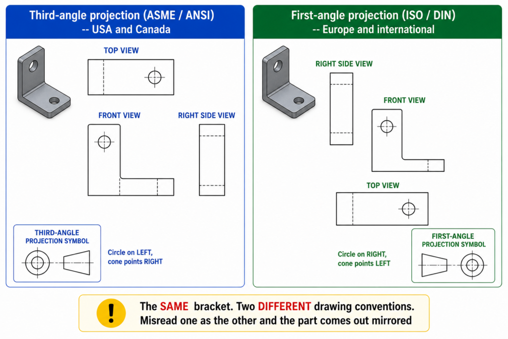
    Third-Angle vs First-Angle Projection: The Most Visible Difference

    This is the difference that causes the most obvious manufacturing errors when it is not checked. The projection method determines where each view sits on the drawing sheet relative to the front view, and getting it wrong means reading a right side view where a left side view should be, and vice versa.

    AspectThird-angle projection (ASME / ANSI)First-angle projection (ISO / DIN)
    Where views sitView placed on the side you look from. Right side view sits to the right of front view.View placed on the opposite side. Right side view sits to the LEFT of front view.
    Top view positionTop view sits ABOVE the front viewTop view sits BELOW the front view
    Identification symbolCircle on left, cone pointing rightCircle on right, cone pointing left
    Dominant standardUSA, Canada, Australia (some use)Europe, Asia, rest of world
    Risk of confusionReading first-angle as third-angle produces mirrored or inverted partsSame risk applies in reverse for non-European readers
    Where statedAlways in the title blockAlways in the title block
    Critical checkConfirm before reading any drawing from an unfamiliar sourceNever assume. Always check the projection symbol in the title block first.

    The projection symbol in the title block is small and easy to overlook. It is also the single most important piece of information on the drawing for anyone who has not worked with both systems. An engineer trained exclusively in ASME drawings, reading a European supplier’s first-angle drawing without checking the symbol, will consistently misidentify which side of the part each view shows.

    The manufacturing consequence of projection confusion:  A bracket designed with a mounting boss on the right side, read from a first-angle drawing by an engineer expecting third-angle, will be interpreted as having the boss on the left side. The machinist machines what the drawing appears to show. The part is wrong. By the time it is discovered, the setup, material, and machining time are wasted. The root cause is not the drawing. It is failing to check the projection symbol before reading the views.

    Envelope vs Independency: The Most Important Technical Difference

    This is the difference that causes the most subtle and expensive manufacturing problems when standards are mixed, because the same tolerance value means something different depending on which principle applies. A 25mm shaft toleranced at plus or minus 0.1mm under ASME and the same shaft under ISO are not the same specification, even though the numbers are identical.

    AspectEnvelope Principle (ASME Y14.5)Independency Principle (ISO 8015 / DIN)
    What it meansThe size tolerance automatically controls form. A 25mm +/-0.1mm cylinder may not exceed a perfect 25.1mm envelope at any cross-section.Size and form are independent. A 25mm +/-0.1mm cylinder may be anywhere between 24.9mm and 25.1mm at any cross-section, but form errors must be separately controlled.
    Who controls form errorsThe size limits do this automatically for ASME drawings without extra symbolsForm errors (straightness, cylindricity, flatness) must be explicitly called out with GD&T symbols
    Effect on designFewer symbols needed for simple prismatic featuresMore symbols required to fully constrain form, but intent is more explicit
    Effect on inspectionEnvelope gauge checks form and size simultaneouslyForm and size inspected separately unless combined control is explicitly stated
    Which standard appliesASME Y14.5 (default, unless E modifier reverses it)ISO 8015 (default for ISO drawings). ASME can invoke ISO 8015 using the E modifier.
    Risk of misinterpretationAn ISO-trained inspector may not apply the envelope check on an ASME drawingAn ASME-trained inspector may assume form is controlled when it is not on an ISO drawing

    A Practical Example of the Difference

    An ASME drawing specifies a shaft diameter of 25.00mm plus or minus 0.10mm. Under the envelope principle, this means the shaft must pass through a perfect 25.10mm ring gauge (the maximum material boundary) and must be no smaller than 24.90mm anywhere. The ring gauge check automatically verifies that the shaft is straight and circular within the size tolerance. No separate cylindricity callout is needed.

    The same shaft on an ISO GPS drawing with the same diameter tolerance of 25.00mm plus or minus 0.10mm operates under the independency principle. The shaft may be anywhere between 24.90mm and 25.10mm at any cross-section, but the form errors (how straight and circular it is) are not controlled by the size tolerance. If the shaft must also be straight within a certain tolerance, a separate straightness callout is required. If cylindricity must be controlled, a cylindricity callout is required.

    GD&T principles comparison Envelope Principle vs Independency Principle
    The envelope vs independency difference is invisible on the drawing unless you know which standard applies.
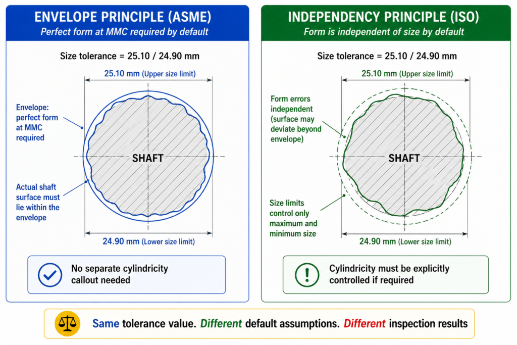
    The practical result: a shaft manufactured to the ASME specification may have better form control than required by ISO, or an ISO shaft may have worse form than an ASME-trained inspector expects. Both are correct for their respective standards. Neither is wrong. But if an inspector trained in ASME applies the envelope principle to an ISO-drawn part, they may accept or reject parts incorrectly.

    GD&T Symbol Differences Between ASME and ISO: Where Conflicts Actually Live

    Most are identical between ASME Y14.5 and ISO 1101. The flatness symbol, the straightness symbol, the angularity symbol, the position symbol: all use the same geometric shapes with the same meaning. This convergence has been deliberate and sustained over decades of parallel standard development. The conflicts that exist are important precisely because they are not obvious from a visual scan of the symbols.

    Feature / SymbolASME Y14.5ISO GPS (ISO 1101)Practical consequence of mixing
    FlatnessFlatness symbol (parallelogram)Same symbol, different default scopeBoth use same symbol but ISO requires explicit callout where ASME uses envelope rule
    CylindricityExplicit callout requiredExplicit callout requiredNo difference in symbol, significant difference in when it is needed
    Position (Location)True position symbol, bidirectionalSame symbol, ISO may use differentlyAlways verify datum scheme matches between supplier and buyer
    Datum feature symbolFilled triangle on leaderSame but triangle placement differsDatum A may point to different surface if convention not stated
    AngularityAngularity symbolSame symbolNo symbol conflict, same interpretation
    ConcentricityIn ASME Y14.5-2018: deprecatedStill used in ISOCritical conflict: ASME has removed this symbol. ISO still uses it.
    SymmetryIn ASME Y14.5-2018: deprecatedStill used in ISOCritical conflict: same as concentricity situation above.
    RunoutCircular and total runoutCircular and total runoutSame meaning, same symbols, no conflict
    Projected tolerance zonePTZ modifier in ASMEISO uses P modifier differentlyPTZ application differs between standards. State standard on drawing.
    Surface texture (Ra)ASME B46.1ISO 1302 / ISO 4287Both use Ra value but measurement method and filtering can differ

    The Concentricity and Symmetry Deprecation: A Live Conflict

    The most significant current conflict between ASME and ISO GD&T symbol sets is the deprecation of concentricity and symmetry in ASME Y14.5-2018. These symbols remain in active use in ISO GPS drawings and are taught in ISO-based GD&T training globally.

    In ASME Y14.5-2018, both were removed and replaced by position or profile of a surface controls, which Subcommittee 5 argued were more precisely defined and more readily inspectable. The argument has merit: concentricity as defined required deriving a median point from every diametrically opposed pair of points on the surface, which is mathematically rigorous but metrologically challenging.

    The practical consequence for engineers: if you receive a drawing with a concentricity symbol and you are working to ASME Y14.5-2018, the symbol is formally undefined in your standard. If the drawing states ISO 1101 as its reference, the symbol is valid and means what it says. If the drawing states nothing, you have no way of knowing which interpretation to apply without asking. This is exactly the situation the title block note requirement is intended to prevent.

    Key Engineering Drawing Standards: Complete Reference Table

    The table below provides a quick reference to the most important engineering drawing standards across all three systems, covering what each standard covers and its current status.

    StandardBodyYear / StatusWhat it covers
    ASME Y14.5ASME2018 (R2024)Geometric dimensioning and tolerancing: all GD&T symbols, datum references, tolerance zones
    ASME Y14.1ASMECurrentDrawing sheet sizes, title block format, and drawing format requirements
    ASME Y14.2ASMECurrentLine conventions and lettering for engineering drawings
    ASME Y14.41ASMECurrentDigital product definition data practices (MBD, 3D annotation)
    ASME Y14.100ASMECurrentEngineering drawing practices: completeness, approval, revision control
    ISO 128ISOISO 128-1:2020General principles for technical drawings: line types, projections, views
    ISO 1101ISOISO 1101:2017Geometrical tolerancing: symbols, definitions, tolerance zones (ISO GPS core standard)
    ISO 8015ISOISO 8015:2011Fundamentals of tolerancing: independency principle, ISO default rules
    ISO 2768ISOISO 2768-1/2General tolerances for linear and angular dimensions (medium m, fine f classes)
    ISO 7200ISOISO 7200:2004Title block format and data fields for technical drawings
    ISO 1302ISOISO 1302:2002Surface texture indication on technical drawings (Ra, Rz symbols)
    ISO 10628ISOISO 10628-2:2012Symbols for process plant diagrams (P&IDs and flow diagrams)
    DIN 6771DINCurrentGerman title block standard, supplementary to ISO 7200
    DIN ISO 1101DINMirrors ISO 1101German national adoption of ISO geometrical tolerancing standard
    DIN 7168DINCurrentGerman general tolerances for linear and angular dimensions (precedes ISO 2768)
    DIN EN ISO 2768DINCurrentGerman adoption of ISO 2768 general tolerances, often still cited as DIN 2768
    Practical rule for cross-border drawings:  When creating a drawing that will be manufactured outside your home country, look up whether the standards you are referencing are recognised by your supplier’s standards system. Most ASME standards are not formally adopted in Europe. Most ISO standards are available in the USA but not universally taught or enforced. When in doubt, state all relevant standards explicitly in the general notes and confirm with the supplier’s quality team that they hold the referenced documents.

    General Tolerances: ISO 2768, DIN 7168, and the ASME Approach

    General tolerances are the tolerances that apply to all undimensioned or untoleranced features on a drawing, defined by a single title block reference rather than individual callouts. They are one of the most frequently misunderstood elements of cross-standard drawing practice.

    ISO 2768: The International General Tolerance Standard

    ISO 2768 defines general tolerances for linear and angular dimensions in two parts. ISO 2768-1 covers linear dimensions and angles in four classes: fine (f), medium (m), coarse (c), and very coarse (v). ISO 2768-2 covers geometrical tolerances in three classes: H, K, and L. A drawing referencing ISO 2768-mK in its general notes is specifying medium-class linear tolerances and K-class geometrical tolerances for all features not individually dimensioned.

    ISO 2768 medium (m) is the most commonly specified class for general machined parts and represents what most competent machine shops can hold in production without special process controls. Fine (f) requires tighter process discipline and is appropriate for precision assemblies. The class should be chosen to match the actual manufacturing process capability of the supplier, not to the tightest possible requirement.

    DIN 7168 and DIN 2768: The German Predecessors

    DIN 7168 is the German general tolerance standard that predates ISO 2768 and covers similar ground with some different tolerance class definitions. Many older German engineering drawings reference DIN 7168 rather than ISO 2768. The two are not identical in all tolerance class values, which means a drawing referencing DIN 7168 fine and a drawing referencing ISO 2768-f are not necessarily specifying the same tolerances on every feature.

    DIN 2768 is frequently cited in engineering contexts but refers to the German national adoption of ISO 2768, technically designated DIN EN ISO 2768 in its current form. For practical purposes, DIN EN ISO 2768 and ISO 2768 are technically equivalent. DIN 7168 is the historically distinct German standard that should not be assumed equivalent to ISO 2768 without checking the specific tolerance values.

    ASME and General Tolerances

    ASME does not use ISO 2768. The ASME approach to general tolerances is different: ASME Y14.5 provides for general tolerance notes in the title block that define plus/minus values for specific dimension ranges, and ASME Y14.100 covers drawing practices including default tolerances. An ASME drawing with a title block note reading ‘3-place decimals: plus/minus 0.005 inch’ is applying a general tolerance, but under a completely different framework from ISO 2768.

    An engineer moving from an ISO GPS environment to an ASME environment cannot assume that referencing ISO 2768 is meaningful on an ASME drawing. It is not part of the ASME drawing practice system. The general tolerances must be expressed using ASME-compatible notation.

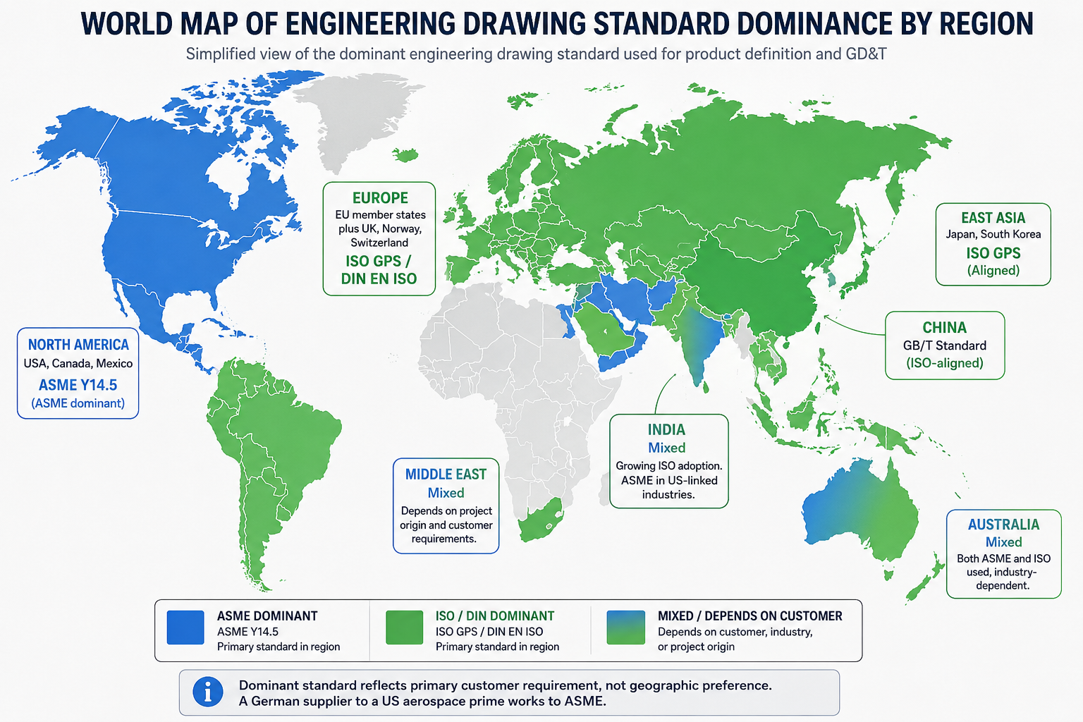
    Which Industries Use Which Standards: The Real-World Map

    Standard selection in most organisations is driven by customer requirements, regulatory obligations, and the geographic location of the primary manufacturing base, not by any abstract technical preference. Understanding which standards dominate which industries tells you immediately which standard to use for a given project.

    IndustryDominant standardReasonTypical supplementary standards
    US Aerospace and DefenceASME Y14.5-2018MIL-STD heritage, US OEM requirementAS9100, ASME Y14.100, ASME Y14.41 for MBD
    European AerospaceISO GPS (EN 9100 aligned)EU OEM and EASA regulatory chainISO 10135, ISO 1302, NADCAP quality reqs
    German Automotive (VDA)DIN / ISO GPS + VDA normsVDA 2 quality and DIN tool standardsVDA 2, VDA 6.1, DIN 7168, DIN ISO 2768
    US Automotive (AIAG)ASME Y14.5 + AIAGBig-Three OEM supply chain standardAIAG PPAP, MSA, FMEA documentation
    Medical devices (FDA)ASME or ISO by choiceFDA 21 CFR Part 820 references bothISO 13485, FDA guidance on drawings
    Pharmaceutical (EU GMP)ISO GPS preferredEU GMP and EMA regulatory alignmentEU GMP Annex 15, ISO 9001
    Industrial machineryISO / DIN (Europe)EN machinery directive complianceISO 4156, DIN 7168 general tolerances
    Consumer electronicsISO or ASME by regionDepends on where manufactured / soldIPC standards for PCB, ISO 2768 general
    Oil and gas (ASME PCC)ASME B31, API standardsASME pressure vessel and piping codesAPI 6A, ASME B16.5, ASME VIII Div 1

    The US Dominance of ASME in a Global Market

    The survey data from GD&T educator Alex Krulikowski, with 133 respondents from 27 countries, found that 86 percent of US participants use ASME Y14.5 and 56 percent of international participants also use ASME Y14.5. These numbers reflect the historical dominance of US manufacturing, defence, and aerospace programs in setting supply chain documentation standards globally. A German tier-two supplier working for a US aerospace prime must produce ASME-compliant drawings for that program regardless of what their domestic German customers require.

    The result is that many engineering teams outside the US maintain dual capability: ISO GPS for domestic and European customers, ASME Y14.5 for US and US-primed programs. This is manageable but requires explicit drawing management discipline, because the same part designed to two different standards requires two different drawings, and mixing elements from each into a single drawing creates the type of ambiguity that the shaft example at the beginning of this guide illustrates.

    World Map of Engineering Drawing Standard Dominance by Region

    The Title Block: Where the Standard Is Declared and Why It Must Be

    Every engineering drawing has a title block in the bottom-right corner. That title block is the drawing’s identity document, and it is also where the applicable drawing standard must be stated. Without an explicit standard reference in the title block or general notes, any GD&T on the drawing is ambiguous.

    What the Title Block Must State for Standard Compliance

    • Applicable GD&T standard: ‘Geometric tolerancing per ASME Y14.5-2018’ or ‘Geometric tolerancing per ISO 1101:2017’ — state the standard and the year of issue
    • General tolerance reference: ‘Unless otherwise specified, general tolerances to ISO 2768-mK’ or the equivalent ASME general tolerance note
    • Projection method: The first-angle or third-angle projection symbol — this should be graphic, not text, so it is recognisable internationally
    • Surface texture standard: If Ra values are used: ‘Surface texture per ISO 1302’ or ‘Surface texture per ASME B46.1’
    • Units: Millimetres or inches — never ambiguous, always stated
    • Material standard: The full material specification including the relevant standard (ASTM, DIN, EN, JIS) not just the alloy name

    ASME Y14.1 and ISO 7200: Title Block Format Standards

    ASME Y14.1 defines the drawing sheet sizes and title block requirements for ASME drawings. ISO 7200 defines the data field structure for title blocks on ISO drawings. DIN 6771 is the German supplementary title block standard.

    The field names in a DIN title block are often in German: ‘Werkstoff’ means Material, ‘Massstab’ means Scale, ‘Datum’ means Date, ‘Zeichen’ means Signature. An engineer unfamiliar with German who receives a DIN-format drawing from a German supplier will be able to read all the technical geometry but may misidentify which field contains the material specification versus the scale versus the date. Knowing the key field names in the languages of your main supplier countries is a practical working skill.

    Model-Based Definition: How Standards Apply in 3D Environments

    The engineering drawing is no longer always a 2D sheet. Model-Based Definition (MBD) embeds the tolerances, GD&T callouts, surface finish specifications, and material notes directly into the 3D CAD model as annotations, eliminating the 2D drawing entirely for some workflows.

    Both ASME and ISO have standards for MBD. ASME Y14.41 defines digital product definition data practices, including how 3D annotations are structured, what must be captured in the model, and how the model functions as a design authority without a 2D drawing. ISO 16792 covers the equivalent requirements under the ISO GPS framework.

    The standard selection question does not go away in MBD: it becomes more important, because the software that manages the 3D PMI (Product and Manufacturing Information) must be configured to apply the correct standard’s rules and defaults. CATIA, SolidWorks, NX, and Creo all support both ASME and ISO annotation modes, but the engineer must select the correct mode before applying tolerances to the model. A model annotated in ASME mode and interpreted by a supplier’s software in ISO mode will produce the same misinterpretation as a misread 2D drawing.

    Which Drawing Standard Should You Use? A Decision Framework

    This is the practical question that engineers and engineering managers actually need answered. The decision is not primarily technical. It is driven by the manufacturing context.

    Use ASME Y14.5-2018 when:

    • Your customer is a US aerospace or defence prime contractor
    • Your parts are inspected in the USA under ASME training and tooling
    • Your CAD system is configured with ASME defaults and your team is ASME-trained
    • The supply chain is primarily North American with US-standard inspection infrastructure

    Use ISO GPS (ISO 1101 and GPS family) when:

    • Your customer is European, particularly in Germany, France, Scandinavia, or other ISO-dominant markets
    • Your parts will be manufactured in Asia, where ISO standards are increasingly the baseline
    • The project involves international supply chains across multiple countries
    • Your team has ISO training and your CAD system is configured for ISO annotation

    Use DIN EN ISO when:

    • Your customer or program requires DIN references explicitly (common in German automotive and industrial machinery)
    • You are supplying into German automotive programs requiring VDA supplementary standards
    • The drawing must be formally compliant with German national adoption standards for procurement or regulatory reasons

    When your supply chain crosses standards:

    • State the governing standard explicitly in the title block. Do not leave it implicit.
    • If the drawing will be used by both ASME and ISO-trained engineers, produce two drawing sets or add a clear cross-reference note explaining which standard governs each section.
    • Train your suppliers in the standard you are issuing. Do not assume they know both.
    • Audit supplier inspection equipment and training against the standard you require. Gauges calibrated for ASME inspection may not be valid for ISO GPS inspection requirements.
    The one rule that prevents most cross-standard problems:  State the drawing standard in the title block on every drawing, every time. Not as a company logo or a footer note that gets overlooked. As a mandatory general note: ‘All geometric tolerances to ASME Y14.5-2018 unless otherwise stated.’ A two-second addition to the title block setup prevents the type of shaft rejection scenario described at the start of this guide.

    10 Engineering Drawing Standard Mistakes That Cause Real Manufacturing Problems

    These are the errors that show up most consistently in cross-border drawing reviews, supplier qualification audits, and failure investigations where the root cause traces back to a standards mismatch rather than a design error.

    MistakeConsequencePrevention
    Not stating the drawing standard in title blockManufacturer interprets GD&T under wrong standard. Form controls and datum behaviour differ.Always include a general note: ‘Unless otherwise specified, this drawing is to ASME Y14.5-2018’ or equivalent ISO/DIN reference.
    Reading a first-angle drawing as third-angleParts built with holes and features mirrored or on the wrong faceCheck the projection symbol in the title block before reading any view. Never assume.
    Mixing ASME and ISO symbols on one drawingAmbiguous or conflicting tolerance interpretationCommit to one standard per drawing. If global supply chain requires both, produce two drawing sets.
    Assuming ISO 2768 applies on an ASME drawingISO 2768 is not referenced in ASME. ASME uses its own general tolerance block.State the applicable general tolerance standard explicitly in the title block or general notes.
    Using concentricity from ISO on an ASME drawingConcentricity was deprecated in ASME Y14.5-2018. Coaxiality is now defined via position or profile.Use ASME-compliant controls for coaxiality: true position relative to datum axis, or profile of a surface.
    Assuming DIN 2768 and ISO 2768 are identicalThey are not. DIN 7168 and DIN 2768 have different tolerance classes and some different values.Check the exact DIN standard referenced on the drawing. Do not assume ISO equivalence without verification.
    Applying the independency principle to an ASME drawingForm errors are not separately controlled on ASME drawings by default. The envelope rule applies.For ASME drawings, if you need form independent of size, add the circle-E modifier explicitly to invoke independency.
    Ignoring the title block language on international drawingsDIN drawings from German suppliers will use German abbreviations (Werkstoffe, Massstab, Datum, Zeichen)Learn the key title block field names in the languages of your main supplier countries.
    Specifying Ra surface finish without stating the standardRa values are measured differently under ASME B46.1 and ISO 4287. The number is not directly comparable.State the applicable surface texture standard alongside the Ra value. Ra 1.6 per ISO 4287 is different from Ra 1.6 per ASME B46.1.
    Using old DIN standards superseded by ISO adoptionsOld DIN-only standards may reference values not in use at the supplierCheck whether the DIN standard cited has been replaced by a DIN EN ISO version. Many have since the 1990s harmonisation.

    Conclusion:

    The purpose of engineering drawing standards is to create a shared language between the person who designs a part and the person who makes or inspects it. ASME Y14.5, ISO GPS, and DIN standards all achieve this goal within their respective domains. The problems arise at the boundaries: when a drawing produced in one standard travels to a reader trained in another.

    The technical differences between ASME and ISO GPS are real and significant: the envelope vs independency principle changes what a size tolerance means. The deprecation of concentricity and symmetry in ASME Y14.5-2018 creates a live conflict with ISO GPS. The projection method difference produces mirrored or inverted parts if not checked. None of these differences are obscure. All of them are well-documented in the respective standards. The problem is that they only become visible at the moment the wrong assumption is applied to the wrong drawing.

    The prevention is straightforward: state the applicable standard in the title block. Check the projection symbol before reading views on an unfamiliar drawing. Never assume that the same symbol means the same thing under a different standard without verifying. And when working across standards in a global supply chain, treat the standards gap as a project risk to be managed explicitly, not a detail to be resolved by whoever is holding the drawing when the question arises.

    State the standard. Check the projection. Verify the defaults. Every time.

    Frequently Asked Questions

    What is the difference between ASME and ISO engineering drawing standards?

    ASME standards, primarily ASME Y14.5, govern engineering drawings in the USA and North America and use third-angle projection. ISO standards, the GPS (Geometrical Product Specifications) system centred on ISO 1101, are the international standard used in Europe, Asia, and globally, and use first-angle projection. The most significant technical difference is tolerancing philosophy: ASME uses the envelope principle where size controls form by default, while ISO GPS uses the independency principle where form must be explicitly controlled with separate symbols. Some GD&T symbols also differ: concentricity and symmetry were deprecated in ASME Y14.5-2018 but remain in use under ISO.

    What does DIN stand for in engineering drawings?

    DIN stands for Deutsches Institut fur Normung, which is the German Institute for Standardization. DIN standards for engineering drawings have been largely harmonised with ISO since the 1990s, and most current DIN drawing standards are cited as DIN EN ISO, meaning the German national adoption of an international ISO standard. DIN standards remain particularly influential in German automotive supply chains (VDA requirements), precision machinery, and industrial equipment sectors where German-originated specifications are common.

    What is third-angle vs first-angle projection on an engineering drawing?

    Third-angle projection is used on ASME and ANSI drawings, primarily in the USA. In third-angle, each view is placed on the same side as the direction you are looking from: the top view sits above the front view, and the right side view sits to the right. First-angle projection is used on ISO and DIN drawings, primarily in Europe and Asia. In first-angle, each view is placed on the opposite side: the top view sits below the front view, and the right side view sits to the left. A small symbol in the drawing title block identifies which projection is used. Misreading one as the other produces parts with features on the wrong faces.

    What is the envelope principle in ASME Y14.5?

    The envelope principle, also called the Taylor principle, is ASME Y14.5’s default rule for size tolerances. It states that the size tolerance limits of a feature also control the maximum variation in form. A shaft with a diameter tolerance of 25mm plus or minus 0.1mm cannot exceed a perfect cylinder of 25.1mm diameter at any cross-section. This means size tolerances implicitly control straightness and circularity without requiring additional GD&T symbols. ISO GPS uses the opposite default: the independency principle, where size and form errors are controlled independently. ISO requires explicit GD&T callouts to control form even on simple sized features.

    Which drawing standard is used in aerospace?

    US aerospace programs follow ASME Y14.5-2018 as the primary GD&T standard, supplemented by ASME Y14.100 for drawing practices and ASME Y14.41 for Model-Based Definition. European aerospace programs follow ISO GPS standards aligned with EN 9100 quality requirements. Multinational programs, such as those where US OEMs work with European suppliers, sometimes require drawings to comply with both, which is one of the most challenging aspects of global aerospace supply chain management. The drawing must explicitly state which standard applies to avoid ambiguity.

    Can ASME and ISO GD&T symbols be used on the same drawing?

    Mixing ASME and ISO GD&T symbols on the same drawing without explicit notation creates serious risk of misinterpretation because the same symbol can mean different things under different standards, and default assumptions differ significantly. Concentricity is a direct example: the symbol exists in ISO but has been deprecated in ASME Y14.5-2018. If a drawing must be used in both ASME and ISO manufacturing contexts, the safest approach is to produce two separate drawing sets, one referencing each standard, or to add a prominent general note specifying which standard governs all GD&T callouts.


    asme.org/codes-standards/find-codes-standards/y14-5-dimensioning-tolerancing

  • What Is Design for Manufacturability (DFM) and How Does It Affect Your CAD Drawings?

    What Is Design for Manufacturability (DFM) and How Does It Affect Your CAD Drawings?

    10x  cost multiplier at each development stage for fixing the same manufacturing issue. A sketch-stage fix costs hours. A post-tooling fix costs months and six figures.
    1981  year the first DFM software was released on an Apple II Plus, offering real-time feedback to engineers. DFM as a discipline predates the modern CAD era.
    30-50%  typical quote price reduction achievable by applying DFM to sheet metal and machined parts before issue to suppliers (published fabrication industry data, 2026)
    Weeks to days  DFM review cycle time compression reported by CoLab AutoReview users by sharing designs with manufacturing and quality engineers simultaneously, without requiring CAD access

    Introduction:

    There is a particular type of engineering problem that happens quietly, costs a lot, and is almost entirely avoidable. An engineer spends three weeks building a detailed CAD model. The drawing is clean, well-dimensioned, and geometrically precise. It goes to the fabricator. A week later, the quote comes back with a price that is 40 percent higher than expected and a list of queries about features the machinist cannot make with standard tooling.

    Or worse: the drawing passes quoting, the parts are made, and the first batch comes back with features that are technically within drawing tolerance but functionally wrong because the drawing was not specific enough about what the manufacturing process needed to deliver.

    Both of these problems have the same root cause: the design was completed without Design for Manufacturability applied. The engineer knew what the part needed to do. They did not build the knowledge of how it would be made into the decisions that shaped the geometry, the tolerances, and the drawing notes.

    This guide explains what DFM is, how it changes the specific content of CAD drawings, what the most important rules are for each common manufacturing process, how tolerances should actually be allocated rather than how they usually are, what AI DFM tools are doing differently in 2026, and the ten mistakes that most consistently make parts expensive, slow, or wrong.

    Quick definition:  Design for Manufacturability (DFM) is the practice of designing parts and assemblies so they can be manufactured efficiently, at minimum cost, and without the defects that result from ignoring process constraints during design. Applied to CAD drawings, DFM changes how features are geometrically defined, how tolerances are allocated, and what notes and specifications the drawing must contain to produce a manufacturable part.
    What Is Design for Manufacturability (DFM) and How Does It Affect Your CAD Drawings
    DFM is not about making the drawing more complex. It is about making the geometry actually manufacturable.

    What Is Design for Manufacturability? The Clear Explanation

    The idea behind Design for Manufacturability is straightforward. Every manufacturing process has constraints. CNC milling cutters are round, so they cannot cut perfectly sharp internal corners. Injection moulds open and close in a single direction, so walls must have draft to release cleanly. Sheet metal presses bend material in a way that deforms nearby holes if they are too close to the bend line.

    DFM is the practice of knowing these constraints and designing around them from the start, rather than discovering them when the quote comes back with a problem list or when the first batch fails inspection. It is not a single review step at the end of the design process. It is a continuous mindset applied to every feature as the model is built.

    The core disciplines within the broader DFM umbrella include:

    • DFM (Design for Manufacturability): individual part geometry designed to be made efficiently by the target process
    • DFA (Design for Assembly): assemblies designed to be assembled with minimum parts, minimum operations, and mistake-proof orientations
    • DFMA (Design for Manufacture and Assembly): both combined, which is how most mature organisations approach the methodology
    • DFQ (Design for Quality): geometry and tolerances designed so that inspection and quality control are practical and reliable
    • DFS (Design for Sustainability): material selection and geometry designed for minimum material waste, energy use, and end-of-life disassembly

    This guide focuses on DFM in its most direct engineering application: how the manufacturing process a part will go through should determine the geometry, tolerances, and documentation of the CAD drawing that produces it.

    Why DFM Has Been Around Since 1981 and Still Gets Ignored

    The first DFM software was released in 1981 on an Apple II Plus. Boothroyd Dewhurst, Inc. was founded in 1983 to commercialise DFM and DFA methodology. The principles have been taught in mechanical engineering degrees for four decades. And yet, the most common feedback from manufacturing engineers reviewing designs from product engineers is still that basic DFM rules have not been applied.

    The reason is structural, not individual. In most product development workflows, the design engineer and the manufacturing engineer are separated by process, timeline, and sometimes by geography. The design engineer’s incentive is to get the design right functionally. The manufacturing engineer’s knowledge enters the process only at review gates that happen after significant design investment has been made. By the time a DFM problem is formally identified, it is expensive to fix.

    AI DFM tools in 2026 are beginning to solve this by giving the design engineer manufacturing feedback at the moment they are making the decisions that create the problem, not after those decisions are locked into a finished drawing.

    The Cost of Getting DFM Wrong: Why Early Matters So Much

    The relationship between when a manufacturing problem is discovered and what it costs to fix it is not linear. It is exponential. Published data from the manufacturing industry consistently shows a ten times cost multiplier at each stage of the development process.

    StageWho catches the issueTypical correction costTime impact
    Concept / sketchDesign engineerNear zero: edit the sketchHours
    CAD model completeDFM review or tool$1,000 – $5,000Days to 1 week
    Drawing issuedManufacturer or DFM check$5,000 – $20,0001-3 weeks
    Prototype builtTesting team$20,000 – $100,000Weeks to months
    Tooling cut or orderedProduction engineer$50,000 – $500,000+Months
    Volume productionQuality / customer return$500,000 – millionsProgramme delay

    These are not theoretical figures. They reflect the actual economics of product development: engineering time to redesign, management overhead to approve the change, supplier communication to revise the order, scrapped tooling or scrapped parts, extended lead times, and in volume production, the cost of customer returns and warranty claims.

    The table makes the business case for DFM review at the concept stage self-evident. The cost of an engineering hour at concept is the same as at prototype. But an engineering hour at concept prevents a problem that would cost a hundred times more to fix at the same stage one step later in the process.

    The most common DFM timing mistake:  Treating DFM as a drawing release gate rather than a design activity. When DFM review only happens after the CAD model is complete and the drawing is drafted, every finding requires changes to finished work. The model must be reopened and edited. The drawing must be revised and re-checked. If DFM is instead applied feature by feature as the model is being built, the cost of each correction is essentially zero because the geometry does not yet exist in final form.
    Cost of Design Change by Development Stage Bar Chart
    DFM is not about adding cost to the design process. It is about avoiding the far larger costs that come when manufacturing problems are discovered late

    How DFM Directly Affects Your CAD Drawings: Element by Element

    The clearest way to understand how DFM in CAD works in practice is to look at specific drawing elements and compare how they appear with and without DFM applied. The differences are not cosmetic. They are the difference between a drawing that a manufacturer can confidently execute and one that generates a query list before production starts.

    Drawing ElementWithout DFM thinkingWith DFM applied
    Internal corner radiusSharp 90-degree corners on pocketed featuresMinimum radius callout matching available tool size
    Draft anglesVertical walls on moulded or cast parts1-3 degree draft on every wall with draw direction arrow
    TolerancesUniform tight tolerance on all featuresSelective: tight on functional interfaces, ISO 2768 elsewhere
    Wall thicknessVariable wall, thicker for stiffness, thinner for weightUniform wall, stiffness achieved through ribs and form
    Hole placementHoles positioned by assembly need aloneHoles checked against DFM rules for process before finalising
    Surface finishSingle Ra value across all surfacesSurface finish specified by zone: mating, sealing, general
    Material calloutNominal material grade, no processing specFull material spec with temper, condition, and standard reference
    Weld symbolsGeneric weld calloutProcess-specific: groove type, joint prep, inspection class
    GD&TAll dimensions in plus/minusGD&T applied at functional interfaces, datum structure defined
    NotesGeneric manufacturing notesProcess-specific notes: tool access, assembly sequence, inspection

    The Tolerance Conversation: What Most Engineers Get Wrong

    Tolerance over-specification is one of the most consistently expensive DFM failures, and one of the most consistently overlooked. When a drawing applies the same tight tolerance to every dimension regardless of whether that dimension affects function, the fabricator must either meet every tolerance at premium cost or query the drawing. Most of the time, tight tolerances are applied by default because the engineer did not consciously decide what each feature’s tolerance should be.

    The correct approach is selective tolerancing: apply tight tolerances only to features that genuinely require them for assembly or function, and let everything else default to a general tolerance standard like ISO 2768 medium (m). This approach communicates clearly to the fabricator what is critical and what is not, allowing them to prioritise process control where it matters and use their judgment elsewhere.

    Feature typeStandard tolerancePrecision toleranceWhen to specify precision
    Non-functional dimensionsISO 2768-mNot neededNever. Leave to process default.
    Mating clearance fitsISO 2768-mH7/g6 or similarWhen assembly requires controlled clearance
    Press fits / interferenceISO 2768-fH7/p6 or tighterWhen retention force is load-bearing
    Bearing seatsIT6-IT7 typicalIT5 for precisionAll rotating or oscillating bearing interfaces
    Sealing surfacesRa 1.6 surface finishRa 0.8 or 0.4All elastomeric or metal-to-metal seals
    Bolt clearance holesH12 or H13Not neededOnly for precise pin/dowel location
    General machined facesISO 2768-mAvoidGeneral form only, not functional mating
    Welded joint gapsPlus/minus 1.0mmPlus/minus 0.5mmOnly for precision structural weld joints
    The tolerance audit habit:  Before releasing any drawing, go through every toleranced dimension and ask one question: does the function of this part or assembly change measurably if this dimension is at the opposite end of its tolerance? If the answer is no, the tolerance is over-specified. Remove it or replace it with a general note reference. This single habit reduces manufacturing cost on most parts by 10 to 30 percent without changing function.

    DFM Rules by Manufacturing Process: What the Drawing Must Communicate

    The most important DFM knowledge for a design engineer is process-specific. The rules for CNC machining DFM are different from the rules for injection moulding, which are different from sheet metal, which are different from casting. The manufacturing process determines what the drawing must say, and a drawing that does not communicate the right things for its intended process is not a complete engineering document.

    Manufacturing ProcessKey DFM Rules for CADCommon CAD drawing violations
    CNC MachiningMin internal corner radius = tool radius + 10%. Max depth-to-width = 4:1 for slots. Uniform wall thickness. Limit setups to one or two sides.Sharp internal corners, pockets deeper than tool reach, features requiring 5-axis where 3-axis is spec
    Injection MouldingDraft angle 1-2 degrees on all walls. Min wall 1.2mm, uniform thickness. Rib height max 3x wall thickness. Gate location away from mating faces.No draft on tall walls, variable wall thickness causing sink marks, undercuts needing side actions
    Sheet MetalMin hole diameter = material thickness. Hole-to-bend distance = 2.5x thickness. Flange height = 4x thickness. Bend relief at intersecting bends.Holes too close to bends, flanges too short for press brake, no bend relief at corners
    Die CastingDraft 1-3 degrees. Wall uniformity critical. Parting line position chosen to minimise surface marks. Draft on cores and inserts.Non-uniform walls causing porosity, draft violations, undercuts on parting plane
    3D Printing (FDM)Orient to minimise supports. Min feature 2x nozzle diameter. Avoid horizontal overhangs beyond 45 degrees. Bridge length under 50mm without support.Features requiring excessive support, thin horizontal bridges, tolerance expectations beyond FDM capability
    Casting (sand/invest.)Min wall 3-5mm depending on alloy. Generous draft 2-5 degrees. Avoid sharp transitions, use fillets everywhere. Core placement feasibility.Thin sections that cannot fill, missing draft, sharp corners causing stress concentration in casting
    Welded fabricationAccess for welding torch and visual inspection. Joint gap specification. Weld sequence to minimise distortion. Avoid welds in high-stress zones.No access for torch, joints requiring simultaneous multi-position welding, tolerance on welded geometry too tight
    Turning / lathe workConsistent diameters to minimise tool changes. Undercuts need relief groove. Chamfers on all transitions. Length-to-diameter max 4:1 without steady.Long slender parts with no steady provision, multiple non-standard diameters, undercuts without relief

    CNC Machining DFM: The Internal Corner Is Where It Always Breaks

    The single most common CNC machining DFM violation is the sharp internal corner in a pocketed feature. A milling cutter is round. It cannot cut a 90-degree internal corner. It leaves a radius equal to its own radius. If the design requires a sharp corner, either a different operation is needed (EDM wire cutting, broaching, or grinding), or the part cannot be made as drawn.

    The solution is not complicated: specify a minimum internal corner radius in every pocketed feature, equal to the cutter radius plus ten percent clearance. For a 10mm end mill, specify R6mm internal corners. For a 6mm end mill, R4mm. If the mating part that fits into the pocket has a sharp corner, chamfer or relieve that part’s corner rather than requiring the pocket to be square.

    The second most common issue is feature depth relative to available tooling. Standard end mills have a flute length to diameter ratio of around 3:1 to 4:1. A pocket 60mm deep requiring a 10mm end mill cannot be machined with standard tooling because the flute length is only 30 to 40mm. The feature requires special extended-reach tooling, which adds cost, delivery time, and vibration risk to the operation. If the pocket depth is driven by function, acknowledge in the notes that extended tooling is required and confirm with the machinist before releasing.

    Injection Moulding DFM: Draft and Wall Thickness Are Not Optional

    Draft angle is the first and most critical injection moulding DFM rule. When a part is injected into a mould, it must be ejected cleanly as the mould opens. Without draft on the walls, the part grips the mould and either damages the surface, requires excessive ejection force that marks the part, or sticks entirely. The minimum draft angle depends on the surface finish: polished surfaces require at least 0.5 degrees, textured surfaces require 3 to 5 degrees in addition to the texture depth.

    Wall thickness uniformity is the second critical rule. Injection-moulded parts cool from the outside in. Thick walls cool slowly, thin walls cool quickly. Where thick and thin sections meet, the differential cooling creates internal stress, sink marks on the surface opposite the thick section, and warping as the part cools unevenly. The DFM-compliant approach is to design uniform wall thickness throughout and use ribs and gussets to add stiffness, not increased wall thickness.

    Rib design follows specific proportions from the wall: rib height maximum 3 times the wall thickness, rib thickness 50 to 60 percent of the wall thickness, and a draft of 0.5 to 1 degree on each rib face. These proportions prevent the rib from causing sink marks on the visible face while providing the stiffness that the design requires.

    Sheet Metal DFM: The Rules That Are Invisible Until You Break Them

    Sheet metal DFM rules are covered in depth in our guide on sheet metal design for manufacturing. The most consequential rules that affect CAD drawings specifically are the hole-to-bend distance (minimum 2.5 times material thickness from the hole edge to the nearest bend tangent line), the flange height minimum (4 times material thickness for press brake grip), and the requirement for bend relief cuts at all intersecting bends.

    These rules are invisible on the finished drawing to anyone who does not know them. A hole positioned 3mm from a bend in 2mm steel looks like a standard hole. The drawing does not announce that it will deform oval during bending. The experienced fabricator will query it. The inexperienced one will cut it and discover the problem at forming.

    AI DFM Tools in 2026: From Rule Checkers to Active Design Optimisers

    The AI DFM tool landscape in 2026 has split into two distinct categories: tools that check designs against rules and flag problems, and tools that actively optimise designs against manufacturing constraints without requiring the engineer to make every correction manually. Understanding the difference helps set realistic expectations about what each tool can deliver.

    AI DFM Analysis Interface Real-Time Feedback on CAD Model
    I DFM tools in 2026 flag issues as you model, not after the drawing is released. The fix takes seconds. The same fix after tooling takes months.
    ToolTypeWhat it checksCAD integration
    Xometry DFMCloud / uploadCNC, 3D printing, injection mouldingSTEP upload, instant feedback online
    CoLab AutoReviewCollaboration AIBest practices, company-specific standardsComment on 3D models in browser, no CAD needed
    InfinitFormIn-CAD AIActively optimises geometry, not just flagsDirect Fusion 360 and SolidWorks integration
    Autodesk DFM (Fusion)In-CAD integratedMachining, additive, sheet metalNative in Fusion 360 Manufacture workspace
    DFMXpressIn-CAD integratedMachining and injection moulding rulesNative in SolidWorks, runs on active model
    Dashnode AI DFMCloud / uploadCNC, turning, sheet metal, additiveSTEP/IGES upload, detailed feature-level report
    Protolabs DFMCloud / uploadInjection moulding, machining, 3D printingPart upload on quoting platform
    Fictiv DFM feedbackCloud / uploadAll common processes with manufacturabilityIntegrated in quoting and ordering workflow

    Static Rule Checkers vs AI-Driven Optimisers

    Traditional DFM tools, including the built-in DFMXpress in SolidWorks and early versions of cloud upload tools, apply static geometric rule sets. The rules are hard-coded: minimum corner radius, minimum draft, minimum hole diameter. When a feature violates a rule, the tool flags it. The engineer decides what to do.

    The limitation identified in a March 2026 CoLab analysis is that static rule checkers often generate high volumes of false positive alerts on designs that are technically acceptable for the specific tooling and process setup being used, even if they violate a generic rule. Engineers begin ignoring the alerts because too many are irrelevant. The signal-to-noise ratio degrades the value of the tool.

    AI-trained tools like InfinitForm and the newer generation of analysis engines trained on real manufacturing outcomes are beginning to address this. Rather than applying static geometric rules, they are trained on historical manufacturing data: which designs were quoted at a premium, which resulted in scrap, which required tool changes or process deviations. The feedback is contextual rather than generic, which reduces false positives and increases engineer trust in the outputs.

    InfinitForm: The Active Optimiser Approach

    InfinitForm represents a conceptually different approach from flagging tools. Rather than producing a list of problems for the engineer to solve, it applies automated geometry corrections directly to the CAD model: rounding corners, adding draft, adjusting wall thickness, all within the CAD environment without requiring the engineer to identify and manually fix each issue.

    For engineering teams processing high volumes of similar part geometries, this approach delivers significant throughput gains. For complex or novel designs where the engineering judgment behind each feature is important, the active optimiser approach needs careful supervision: automated corrections can change the design intent if the optimiser does not understand why a specific geometry exists. The engineer remains responsible for reviewing what the tool has changed.

    Cloud Upload Tools: Xometry, Protolabs, and Fictiv

    The cloud quoting platforms operated by Xometry, Protolabs, and Fictiv have built DFM analysis directly into their quoting workflow. When an engineer uploads a STEP file for a quote, the platform analyses the geometry against the selected process rules and returns both a price and a DFM report in the same response.

    This is probably the most consequentially positioned DFM feedback in any workflow: the engineer receives manufacturing feedback at the exact moment they are deciding whether to proceed with the design. A DFM issue flagged at the quoting stage costs an email and a model revision. The same issue discovered during production at that same supplier costs a production hold and an emergency re-design.

    Design for Assembly: The DFM Dimension That Affects the Whole Product

    If DFM focuses on how individual parts are made, Design for Assembly (DFA) focuses on how those parts come together. The principles are related but distinct, and both have direct effects on what appears on CAD drawings and assembly documentation.

    The Boothroyd-Dewhurst Principles That Still Apply in 2026

    Geoffrey Boothroyd and Peter Dewhurst codified the foundational DFA principles in the 1970s and 1980s. Four decades later, they remain the most consistently useful framework for assembly design decisions in CAD:

    1. Minimise the part count. Every part is a cost: material, manufacturing, inspection, inventory, and assembly time. Ask whether each part can be combined with an adjacent part without losing function. The part count is the single highest-lever driver of assembly cost.
    2. Design parts with unambiguous assembly orientation. If a part can be inserted in the wrong orientation, it will be, eventually, and the consequence will be a field failure or an assembly line stoppage. Use asymmetric geometry or assembly features to make the wrong orientation physically impossible.
    3. Design for top-down assembly. Where possible, design assemblies so each part is added from above and drops into place under gravity. This enables robotic assembly and reduces the number of repositioning steps required during manual assembly.
    4. Minimise fastener count and types. Each different fastener type requires a different tool, a different bin, and a different training requirement. Standardise on a minimum number of fastener types and sizes across a product family.

    How DFA Appears in CAD Drawings

    • Poka-yoke features (asymmetric tabs, locating pins, orientation notches) that make wrong assembly physically impossible
    • Assembly sequence notes specifying the order of sub-assembly and final assembly operations
    • Fastener callouts using the minimum number of standardised types across the assembly
    • Clearance specifications for assembly tool access (screwdriver, spanner, rivet gun)
    • Datum references that are accessible and measurable during assembly, not just during inspection

    Integrating DFM Into Your CAD Modeling Workflow

    DFM is most effective when it is not a separate activity from CAD modeling but a habit embedded in how the model is built. The following approach integrates DFM thinking at each stage of the modeling process without adding a separate review gate that is often compressed or skipped under schedule pressure.

    Before Opening the CAD Software

    The most important DFM decision is often the first one: selecting the manufacturing process. The process determines every subsequent DFM rule that applies. A design engineer who does not know whether a part will be machined, moulded, or fabricated cannot make any sensible geometry decisions because the constraints are completely different for each.

    If the process is not yet fixed, the concept design should use geometry that is agnostic enough to work for at least two candidate processes. Do not design sharp internal corners as a default if the part might be injection moulded, because adding draft later is more disruptive than designing with draft from the start. Use the concept stage to test which process is most appropriate before committing to the geometry that locks the choice.

    During Feature Creation

    Apply the most critical DFM rule for the chosen process to each feature as it is created. For machined parts: never create an internal pocket without specifying the corner radius in the feature. For moulded parts: apply draft before finalising any extruded wall. For sheet metal: check hole-to-bend clearance before placing any hole near a fold line.

    This is not additional work. It is the same modeling time applied with process awareness rather than pure geometry focus. The feature takes the same time to create. The only difference is whether the geometry that is created will need to be reopened and corrected when the DFM check is run after drawing completion.

    At Drawing Creation

    The drawing is where DFM is either confirmed or undermined by tolerances and notes. Three things matter most at the drawing stage.

    First, tolerance allocation: apply the tolerance table approach from earlier in this guide. Tight only where function requires it. General reference everywhere else. Add a general tolerance block in the title block referencing ISO 2768-m so the fabricator knows the default.

    Second, drawing notes: add process-specific notes that the drawing geometry alone cannot communicate. Tool access direction for inspection. Acceptable substitution materials if the primary specification is unavailable. Required testing before acceptance. Any feature that is critical to assembly or safety, marked as such.

    Third, run the AI DFM check before releasing. With tools like DFMXpress in SolidWorks or the Fusion 360 DFM workspace, this takes minutes and catches the geometric violations that might have slipped through modeling. Treat any critical finding as a mandatory fix, not an optional consideration.

    10 DFM Mistakes That Make Parts Expensive, Slow, or Wrong

    These are the DFM failures that come up most consistently across machined, moulded, and fabricated part reviews. Each one has a specific, measurable cost consequence and a straightforward prevention strategy.

    MistakeCost consequencePrevention
    Sharp internal corners in CNC pockets100% rejection or EDM rework: $500-$5,000/partSpecify minimum internal radius = tool radius + 10% in all pocketed features. Put it in the drawing notes.
    No draft on injection-moulded wallsMould tools reworked or part sticks on ejectionApply 1-2 degree draft to all walls in draw direction. Check mould flow simulation before tooling.
    Over-toleranced non-critical featuresQuote 30-50% higher than necessaryApply ISO 2768-m as default. Tighten only mating and functional interfaces. Mark critical dimensions clearly.
    Variable wall thickness in mouldingSink marks, warping, weld lines in productionDesign uniform wall thickness. Add ribs for stiffness. Transition thickness changes with tapered sections.
    Undercuts without side actions budgetedTooling cost overrun by 20-40%Identify all undercuts during DFM review and confirm whether side actions are in tooling budget and lead time.
    Material specified without temperWrong material properties, wrong machinabilityAlways specify full material standard: alloy, grade, temper, condition. Not ‘aluminium’ but ‘6061-T6 per AMS 2770’.
    Feature depth exceeding tool reachSpecial tooling ordered, programme delayedCheck all pocket depths against standard end mill reach ratios (max 4:1 depth:diameter for standard tooling).
    No tool access for inspectionIn-process inspection impossible, defects missedDesign inspection access for all critical features. Confirm measurement method with quality team before drawing release.
    Assembly sequence not consideredParts cannot be assembled in the designed orderBuild assembly sequence into notes. Check that every fastener has access and every sub-assembly can reach its position.
    Ignoring DFM until drawing is completeRework of finalised model is expensive and slowIntegrate DFM checks at the concept and mid-model stage, not as a gate after the drawing is finished.
    The DFM checklist for every drawing release:  Before releasing any CAD drawing: (1) Internal corner radii specified for all machined pockets. (2) Draft angles on all moulded or cast walls. (3) Wall thickness uniform or tapered for injection moulding. (4) Hole positions checked against bend distances for sheet metal. (5) Tolerance callouts reviewed, non-critical features set to ISO 2768-m. (6) Full material specification including temper and standard. (7) AI DFM check run and all critical findings resolved. (8) Assembly sequence and tool access confirmed where relevant. Two minutes of checking here prevents two weeks of rework later.

    DFM and Sustainability: The 2026 Dimension

    Sustainability-focused DFM is the fastest-growing component of the discipline in 2026. Regulatory pressure, customer expectations, and genuine cost savings from material efficiency are driving its adoption in sectors from consumer electronics to industrial equipment.

    Sustainability-focused design for manufacturability applies the same logic as cost-focused DFM: the design decision made at the CAD stage determines the material waste, energy consumption, and end-of-life recyclability of every part produced. Those outcomes cannot be improved significantly once the geometry is fixed and tooling is committed.

    • Material efficiency: topology-optimised geometry removes material from low-stress regions, reducing both part weight and the energy required to produce the raw material
    • Process selection for carbon footprint: machining from solid generates significant swarf waste; near-net-shape forming processes such as forging and casting use materially less input stock for the same output part
    • Fastener-free joining: snap-fit, press-fit, and adhesive-bonded joints reduce the number of dissimilar materials in an assembly, improving recyclability at end of life
    • Recycled material specification: calling out recycled aluminium alloys or post-consumer recycled polymer grades in the material specification is now a viable and often cost-neutral choice on many standard part types
    • Design for disassembly: ensuring that assembled parts can be separated at end of life without destroying either component, by avoiding permanent bonding of dissimilar materials and designing accessible fastener access

    Conclusion:

    The engineers who produce drawings that go directly to manufacture without a problem list are not the ones with the most experience. They are the ones who have internalised the constraints of the processes they are designing for, and who apply those constraints feature by feature as the model is built rather than as a checklist after it is finished.

    Design for Manufacturability is not complicated. The rules for each process are learnable in an afternoon. The tolerance strategy is a decision framework, not a table to memorise. The DFM habits, checking corner radii in machined pockets, adding draft to moulded walls, keeping holes away from bends, take no additional time once they are reflexive.

    What makes DFM expensive to ignore is the compounding cost of discovering problems late. What makes it worth prioritising is the compounding benefit of designs that work the first time: faster first article acceptance, fewer supplier queries, lower quoted prices, and manufacturing teams that trust the drawings they receive.

    In 2026, AI DFM tools from InfinitForm, Xometry, CoLab, and others are making it easier to catch the remaining violations that slip through even experienced design reviews. But the tools only work well on designs that were already being thought about correctly. The AI catches what the engineer missed. It does not replace the engineer thinking about manufacturability while the model is being built.

    Design the process into the part. The process cannot be designed in after the drawing is released.

    Frequently Asked Questions

    What is design for manufacturability (DFM)?

    Design for manufacturability (DFM) is an engineering methodology that ensures products are designed to be manufactured efficiently, reliably, and at minimum cost. It involves applying process-specific design rules during CAD modeling, reviewing geometry against manufacturing constraints before drawings are released, and selecting materials and tolerances that match what the production process can actually achieve. DFM reduces rework, scrap, and tooling corrections by catching problems at the design stage rather than on the shop floor.

    How does DFM affect CAD drawings specifically?

    DFM changes what a CAD drawing must communicate. A DFM-compliant drawing includes minimum internal corner radii that match available tooling, draft angles on moulded and cast walls, hole-to-bend distances for sheet metal, and selective tolerances that are tight only on functional interfaces while leaving the rest to ISO 2768 defaults. The manufacturing process determines what the drawing must say. Without DFM applied, drawings routinely specify features that are impossible for the intended process, tolerances that add cost without functional benefit, and geometry that a fabricator must query or reject.

    When in the design process should DFM be applied?

    DFM should be applied at the concept stage, before detailed CAD modeling begins. The cost of fixing a manufacturing issue increases by roughly a factor of 10 at each development stage. Fixing a DFM issue at concept costs engineering time only. The same problem found after tooling is cut costs tens of thousands to hundreds of thousands of dollars and delays the programme by months. The most effective DFM is not a gate review at drawing completion but a continuous habit of checking each feature against the target process as the model is built.

    What are the most important DFM rules for CNC machining?

    The most critical DFM rules for CNC machining in CAD are: minimum internal corner radius equal to the cutter radius plus ten percent, maximum pocket depth to width ratio of 4:1 for standard tooling, uniform wall thickness to avoid chatter and deflection, feature access from two setups maximum, chamfers rather than sharp edges on all transitions, and thread relief grooves on all threaded sections. Each of these rules is directly reflected in how the part is dimensioned and annotated on the drawing.

    What is the difference between DFM and DFA?

    DFM (Design for Manufacturability) focuses on how individual parts are made. DFA (Design for Assembly) focuses on how parts are assembled together. DFM asks whether a single part can be manufactured efficiently by the intended process. DFA asks whether the number of parts can be reduced, whether fasteners are accessible, whether parts can be assembled in only one orientation, and whether the assembly sequence is practical. Both disciplines are related and both affect CAD drawings, but they address different failure modes in product development.

    How does AI DFM analysis work in 2026?

    AI DFM tools in 2026 analyse CAD geometry automatically when a model is uploaded or as it is being built inside the CAD environment. They check features against process-specific rule libraries, flag violations with location, severity, and suggested fix, and in the most advanced tools such as InfinitForm, they automatically optimise the geometry rather than simply flagging the problem. Tools like Xometry and Protolabs integrate DFM feedback directly into the quoting workflow, so engineers receive manufacturability feedback at the same time as they receive a price. The shift from static geometric rules to AI trained on manufacturing outcomes is making DFM analysis faster, more accurate, and more accessible to engineering teams without dedicated DFM specialists.


    Boothroyd Dewhurst: the founding research organisation for DFMA methodology

  • Reverse Engineering Using 3D Scanning: How Physical Parts Become CAD Models

    Reverse Engineering Using 3D Scanning: How Physical Parts Become CAD Models

    $7.51 billion  projected global 3D scanning market size by 2030, growing at 10.1% CAGR from $4.28B in 2024 (Grand View Research)
    0.01mm  best-in-class accuracy achievable with structured light scanning for small precision components in a controlled lab environment
    1/10th the time  Geomagic Design X and Artec claim scan-to-CAD reverse engineering takes one-tenth the time of building the same model from physical measurement alone
    20 seconds  CT segmentation time per scan achieved by AnatomikModeling using VGTRAINER + VGSTUDIO MAX AI, down from 1 hour manually (Hexagon, 2026)

    Introduction:

    A manufacturing plant is called to replace a critical pump impeller. The original manufacturer no longer exists. The engineering drawings were lost in a flood thirty years ago. The only thing available is the worn impeller sitting on the workshop bench.

    Before 3D scanning reverse engineering was available, the options were: manual measurement with calipers and a coordinate measuring machine, which for a complex curved impeller profile could take weeks and still miss detail in the vane geometry; or fabrication by trial and error, which is expensive and slow. Today, an engineer with a structured light scanner and a laptop running Geomagic Design X can have a fully parametric CAD model of that impeller, accurate to 0.02mm, in under a day.

    This is the practical reality of reverse engineering with 3D scanning in 2026. The technology has matured to the point where it is no longer a specialist capability restricted to large aerospace and automotive programs. It is accessible to any engineering team dealing with legacy equipment, worn parts, no-drawing components, or geometry that is simply too complex to measure manually.

    This guide walks through the complete scan to CAD workflow from first capture to exported parametric model, covering what each stage involves, which tools are used, where the process commonly fails, and what AI is beginning to change about a workflow that has traditionally been dominated by skilled human judgment.

    Quick definition:  Reverse engineering using 3D scanning is the process of digitising a physical part into a point cloud with a scanner, converting that data into a clean mesh, and extracting a parametric or surface-based CAD model that can be used for manufacturing, analysis, or modification. The result is a digital model derived from the physical reality of the part, not from original design drawings.
    The Four Stages of Scan to CAD Reverse Engineering
    One physical part. Four processing stages. One parametric CAD model.

    What Is Reverse Engineering with 3D Scanning and Why It Matters

    Traditional engineering goes from design to manufacture: a drawing is created, then a part is made to match it. Reverse engineering inverts that sequence. You start with an existing physical object and work backward to create the design documentation that could have produced it.

    3D scanning makes this process practical for complex geometry. The alternative, manual measurement using calipers, micrometers, templates, and coordinate measuring machines, works adequately for simple prismatic parts with flat faces, cylindrical bores, and standard features. It breaks down for freeform surfaces, complex contours, organic shapes, and any geometry where the critical dimensions are difficult to access with a physical probe.

    When Reverse Engineering Is Actually Needed

    • No surviving drawings: Legacy plant equipment, inherited tooling, or parts from suppliers no longer in business. If the drawings never existed or have been lost, scanning is the only practical route to a CAD model.
    • As-built capture: Where the physical plant or structure has been built and modified over decades in ways that diverge from the original drawings. Oil and gas facilities, ships, and heritage buildings commonly require as-built scanning to support retrofit and maintenance engineering.
    • Worn or damaged part analysis: Understanding how a part has changed from its nominal condition through wear, deformation, or damage. The scan is compared against the nominal CAD model to map deviation.
    • Fitting design to existing geometry: When a new component must fit precisely around or into an existing physical assembly that has no accurate CAD model. Customised prosthetics, ergonomic product design, and retrofit equipment design all rely on this use case.
    • Competitive benchmarking: Understanding how a competitor’s product is constructed by digitising and analysing it. Common in automotive, consumer products, and industrial equipment.
    • Complex freeform geometry: Turbine blades, propeller profiles, automotive exterior panels, injection mould cavities. These surfaces cannot be described accurately by a few measurements. They require full-field 3D capture.

    How 3D Scanners Work: The Physics Behind the Data

    Different scanner technologies use different physics to capture geometry. Understanding the underlying method explains why each type has specific accuracy limits and specific material constraints.

    Structured Light Scanning

    A structured light scanner projects a series of striped or fringe patterns onto the surface of the part. Two cameras observe how those patterns deform as they follow the contours of the surface. The system uses the principle of triangulation: knowing the angle between the projector and each camera, and knowing the expected undistorted pattern, the software calculates the 3D position of every visible point where the pattern deforms.

    The result is a dense, accurate point cloud captured in a single shot or a rapid sequence of shots. High-end systems like the GOM ATOS series achieve accuracies of 0.01mm on small components. This makes structured light scanning the benchmark method for precision part digitisation in metrology and quality control workflows.

    The limitation is field of view: a single setup captures only what the cameras can see. Multiple setups are needed to cover the full part, and all setups must be registered into a single coordinate system. Reference targets, small adhesive dots applied to the part or the fixture, give the registration software fixed points to align the scans against.

    Laser Line Scanning

    A laser line scanner projects a single laser stripe across the surface and records how that line deforms using a camera sensor. The scanner moves relative to the part, sweeping the laser line across the surface to build up a full point cloud. Handheld versions like the Creaform HandySCAN and the Artec Leo use inertial measurement units and surface texture tracking to maintain position without external targets.

    Handheld laser scanning offers significantly more flexibility than structured light for large parts and parts with complex access requirements. Accuracy of 0.05 to 0.1mm is achievable for most mechanical parts with a skilled operator. The penalty relative to structured light is that real-time motion tracking introduces positional noise that the software must manage, and the accuracy degrades slightly as the scanned area grows.

    Photogrammetry

    Photogrammetry uses photographs from multiple positions around an object and computes the 3D positions of identifiable features in those images using the known geometry of the camera. Scale is introduced through coded reference targets of known dimensions. The method is scale-independent: the same technique works for scanning a small artefact on a turntable or a full aircraft fuselage in a hangar.

    Accuracy scales with measurement volume. For a one-metre part, photogrammetry achieves 0.02 to 0.05mm. For a ten-metre structure, accuracy is 0.2 to 0.5mm. The method is particularly strong for capturing overall shape and position with high accuracy across large volumes, and it is often combined with local structured light scanning for features requiring higher local detail.

    CT Scanning: The Internal Geometry Solution

    Industrial CT scanning (computed tomography) is the only widely available non-destructive method that captures internal geometry from a 3D scan. X-rays are passed through the part from multiple angles, and the attenuation of those X-rays through the material is measured by a detector. Software reconstructs the internal and external geometry of the part as a voxel model (a three-dimensional pixel grid) from which a surface mesh can be extracted.

    The method captures everything: external surfaces, internal bores and passages, wall thickness variations, inclusions, voids, and porosity. For cast or moulded parts with critical internal geometry, CT scanning is the only practical option. Published results demonstrate CT scanning reducing CT segmentation from one hour to 20 seconds per scan using AI-accelerated processing in 2026 workflows.

    The limitation is size and cost. CT scanning requires the entire part to fit within the X-ray beam envelope, limiting practical part size to roughly one metre for most industrial systems. Larger parts must be scanned in sections. Cost per scan is significantly higher than optical methods, making CT scanning appropriate for high-value or critical parts where internal geometry is essential, not for routine reverse engineering projects.

    Scanner TypeHow It WorksTypical AccuracyBest ForPrice Range (2026)
    Structured lightProjects fringe patterns, captures deformation0.01-0.05mmSmall-medium precision parts$5k – $80k
    Laser line scannerLaser stripe swept across surface0.02-0.1mmGeneral mechanical parts, panels$8k – $60k
    Handheld laserPortable, marker or markerless track0.05-0.1mmLarge parts, on-site scanning$15k – $80k
    PhotogrammetryMultiple camera angles, targets0.02-0.05mm / metreLarge structures, vehicles, aircraft$5k – $50k
    CT scanning (X-ray)X-ray slices through solid part0.005-0.05mmInternal geometry, complex castings$100k+
    Arm-mounted CMM probeContact probe on articulating arm0.005-0.025mmHigh-precision machined parts$20k – $150k
    LiDAR (long range)Pulsed laser time-of-flight1-5mm at rangeLarge facilities, ships, plant$30k – $200k+

    The Complete Scan to CAD Workflow: Every Stage Explained

    The scan to CAD process for reverse engineering is not a single step. It is a pipeline with nine distinct stages, each requiring specific tools and specific judgment. Understanding each stage prevents the most common failure: assuming a clean part scan automatically produces a usable CAD model.

    Structured Light vs Handheld Laser Scanner Accuracy Comparison
    Scanner selection is an engineering decision. Match the accuracy specification to the tolerance requirement of the part.
    StageWhat HappensKey Software / ToolsCommon Failures at This Stage
    1. PlanIdentify scan coverage, fixturing, targetsPart inspection, scanner spec sheetNot scanning all surfaces, missing undercuts
    2. ScanCapture point cloud from multiple positionsArtec Leo, FARO Arm, Creaform HandySCANNoise from reflective surfaces, gaps in coverage
    3. AlignRegister multiple scan positions to one modelArtec Studio, FARO Scene, VXelementsPoor alignment from insufficient overlap between scans
    4. MeshConvert aligned point cloud to polygon meshArtec Studio, Geomagic Wrap, MeshmixerMesh holes, inverted normals, duplicate faces
    5. CleanRemove noise, fill holes, smooth artefactsGeomagic Wrap, Artec Studio, MeshLabOver-smoothing removes real geometry detail
    6. SegmentIdentify surfaces, features, reference planesGeomagic Design X, PolyWorks, RapidformFeature boundaries misidentified, wrong primitives
    7. ModelFit primitives, extract features, build CADGeomagic Design X, Siemens NX, Creo RENominal model drift from best-fit alignment errors
    8. ValidateCompare model to scan, check deviationsGeomagic Control X, PolyWorks InspectorAccepting deviation above tolerance for critical features
    9. ExportOutput to native CAD formatLiveTransfer to SolidWorks, NX, CATIALosing parametric history during format conversion

    Stage 1 to 4: From Physical Part to Clean Mesh

    The first four stages are about capture and data quality. The planning stage defines the scanning strategy: how many positions are needed, where targets go if required, whether the surface needs preparation, and which scanner is appropriate for the part geometry and required accuracy.

    Surface preparation is frequently underestimated. Reflective metallic surfaces scatter laser and structured light, producing sparse data or complete gaps in the scan. Applying a temporary matte scanning spray, a chalk-based aerosol that wipes clean with a damp cloth, resolves this for almost all metallic surfaces. Dark or black surfaces absorb laser energy with the same result. The spray solution works equally well there. For parts where any surface contamination is unacceptable, switching to CT scanning avoids the problem entirely.

    Mesh cleaning fills the inevitable holes at occluded surfaces, removes noise spikes from scanner artefacts, and repairs duplicate or inverted faces that would cause downstream errors. The principle here is to repair, not to sculpt. The cleaned mesh should represent the real part geometry, not a smoothed approximation of it. Aggressive smoothing removes real geometric detail that the CAD model needs to capture accurately.

    Stage 5 to 7: From Mesh to CAD Model

    This is where the most engineering judgment is applied and where the most time is spent. The cleaned mesh contains the captured geometry but no structural understanding. The software does not know which regions are cylindrical, which are planar, which are filleted transitions. Segmentation divides the mesh into regions that correspond to individual geometric features.

    In Geomagic Design X, this segmentation is increasingly automated: the Feature Wizard identifies prismatic features such as cylinders, planes, cones, and spheres directly from the mesh. For a machined mechanical part, 70 to 80 percent of the features may be identified automatically. The remaining freeform or unusual surfaces require manual region definition.

    Feature extraction fits the best mathematical primitive to each segmented region. A cylindrical region becomes a parametric cylinder with a defined diameter and axis. A planar region becomes a plane with defined orientation. A filleted transition becomes a radius with a defined value. The result is a collection of parametric features that the CAD system can use to build a history-based model, equivalent to what a designer would have built from scratch.

    Stage 8 to 9: Deviation Analysis and Export

    Deviation analysis is the quality gate of the reverse engineering process. The completed CAD model is projected back onto the original scan data and a colour map is generated showing the deviation between the model surface and the scanned surface at every point. Areas of green indicate good agreement within tolerance. Areas of red or blue indicate regions where the model diverges from the scan.

    This analysis identifies whether the model is an accurate representation of the part. For a reverse engineering project, the target deviation depends on the application. A heritage part being reproduced for historical accuracy might accept 0.5mm. A precision aerospace component might require every critical surface to be within 0.02mm. The deviation analysis makes the agreement quantifiable rather than subjective.

    Export uses LiveTransfer technology in Geomagic Design X to send the parametric model directly to SolidWorks, Siemens NX, PTC Creo, Autodesk Inventor, or CATIA with the feature history intact. The receiving engineer can modify dimensions, suppress features, add new geometry, and use the model exactly as they would use a model built originally in that CAD system.

    The one step most engineers skip:  Running the deviation colour map before sign-off. A model that looks right visually may deviate by several tenths of a millimetre from the scan at compound curves and blended transitions. The colour map catches this. Always check the deviation analysis before releasing the model for manufacturing or analysis.
    3D CAD deviation analysis overlay
    The deviation map is the quality proof. Without it, you cannot verify the model matches the part.

    Reverse Engineering Software in 2026: What Is Used and Why

    The reverse engineering software landscape in 2026 is more varied than it has ever been, with traditional established platforms being joined by AI-native tools that automate steps previously requiring significant expert skill. Understanding which tool belongs where prevents expensive mismatches between software capability and project requirement.

    SoftwareDeveloperPrimary FunctionBest For2026 Status
    Geomagic Design XHexagon/3D Sys.Scan to parametric CADMech parts, all industriesIndustry benchmark, Go/Plus/Pro tiers
    Artec Studio 18Artec 3DScan processing and mesh outputArtec scanner ecosystemAI auto-align in Studio 18, 2025
    PolyWorks ModelerInnovMetricPoint cloud to surface and CADLarge industrial partsWidely used in automotive and aero
    Siemens NX RESiemensScan-integrated parametric designAerospace, automotive OEMsDeep NX CAD integration
    CATIA V5/3DE REDassaultScan to Class-A surfaceAutomotive exterior surfacesKey in automotive styling RE
    PTC Creo REPTCScan-aware parametric modelingAerospace, defenceDirect Model tech, no regen needed
    Agisoft MetashapeAgisoftPhotogrammetry to mesh/modelCultural heritage, large objectsLeading photogrammetry pipeline tool
    Recap ProAutodeskReality capture, point cloud mgmtArchitecture, plant as-builtAutodesk cloud-connected, BIM ready
    Backflip AIBackflipAI mesh to parametric CADLegacy part digitisation2025 launch, AI-native, cloud-based
    MeshLab / CloudComp.Open sourcePoint cloud and mesh processingResearch, budget workflowsFree, widely used in academia

    Geomagic Design X: The Benchmark Standard

    Geomagic Design X from Hexagon is the most widely referenced tool for professional scan-to-CAD reverse engineering. Its combination of history-based CAD modeling directly integrated with point cloud and mesh processing sets it apart from tools that either process scans or build CAD models but not both in the same environment.

    The three-tier model introduced in 2026, Go for beginners, Plus for intermediate users, and Pro for full-capability expert workflows, has made the tool more accessible to smaller engineering teams who previously could not justify the full Pro license cost. The LiveTransfer technology, which sends parametric model history directly to the target CAD system without conversion, is the feature that most directly reduces the gap between scan data and a model that can be used productively in the downstream engineering workflow.

    Hexagon also used Geomagic Design X with their HYPERSCAN and MARVELSCAN hardware to create the digital twins of the 2026 Mustang and Camaro, demonstrating that the platform operates at the scale of complete vehicle programs, not just isolated part reverse engineering.

    Backflip AI: The 2026 Disruptor

    Backflip AI, which emerged from stealth in early 2025, represents the most significant new entrant in the reverse engineering software market in years. It uses deep learning to convert raw mesh geometry directly into fully parametric CAD models without the manual feature extraction step that has historically been the most time-consuming part of complex reverse engineering projects.

    For legacy parts with conventional mechanical geometry, cylinders, flanges, bolt patterns, and fillets, Backflip AI can produce a parametric model from a clean mesh in a fraction of the time Geomagic Design X requires with manual guidance. The limitation is complex freeform surfaces where the neural network has less training data and the automatic parametrisation produces less reliable results. For those cases, Geomagic Design X and human expertise remain the stronger choice.

    Scan to CAD Challenges: The Surfaces and Geometries That Make It Hard

    The surfaces and geometries that make 3D scanning reverse engineering difficult are predictable. Knowing them in advance allows the right scanner and preparation strategy to be selected before the project starts, rather than discovering the problem mid-scan.

    ChallengeWhy It HappensPractical Solution
    Reflective surfacesLaser and structured light scatter off mirror finishesApply temporary matte scanning spray. Remove after scanning. Never permanent.
    Black/dark surfacesNear-zero reflectance means no data returnScanning spray again, or switch to CT scanning for fully black parts.
    Thin walls and edgesEdge artefacts and mesh dropout at thin sectionsUse higher-resolution scanner, scan from more angles, reduce scan speed.
    Undercuts and re-entrant geometryLine-of-sight limitation of optical scannersUse CT scanning, or combine multiple scanner positions with rotation fixture.
    Large part with tight local toleranceAccumulated error across full part volumeUse photogrammetry for overall shape, arm-mounted CMM for precise local features.
    Moving or vibrating partsScan data from different positions misalignsRigid fixturing required. Scan in a controlled environment away from vibration sources.
    Internal geometryNo optical access to internal featuresCT scanning is the only non-destructive solution for internal cavities and passages.
    Soft or deformable partsPart shape changes under scanner fixture or gravityUse contact-free scanning with part in service orientation. Minimal fixturing.

    The Reflective Surface Problem in Detail

    Laser and structured light scanners rely on diffuse reflection from the surface to capture point data. A polished or mirror-finish surface reflects the laser at a specular angle that the scanner camera cannot see, producing no data. The practical solution, temporarily applied scanning spray, is so effective and so reversible that it should be the first consideration for any metallic part. The spray dries in seconds, is applied by aerosol, and wipes off completely with a damp cloth.

    The only surfaces where spray cannot be used are those with functional surface properties that must not be contaminated: bearing surfaces, sealing faces, optical components, and parts in clean-room environments. For these, the choice is between CT scanning (which does not rely on surface reflectance) and contact probing with a CMM arm (which bypasses the reflectance problem entirely by touching the surface).

    Where Reverse Engineering 3D Scanning Is Used: Industry Applications

    The applications of reverse engineering with 3D scanning extend across virtually every manufacturing and engineering industry. The common thread is always the same: a physical object exists whose geometry is not fully documented, and that geometry needs to be captured digitally.

    IndustryWhy Reverse Engineering Is UsedTypical Scan Accuracy Required
    AerospaceLegacy part reproduction, maintenance of aged fleet, tooling verification, as-built documentation of complex assemblies0.02-0.05mm for structural, 0.1mm for large structure
    AutomotiveCompetitive benchmarking, clay model digitisation, Class-A surface reconstruction, tooling and die capture0.05mm for body panels, 0.01mm for drivetrain parts
    Oil and gasOffshore plant as-built capture, piping retrofit design, corrosion assessment on aged pipework1-5mm for layout, 0.1mm for flange interfaces
    Medical devicesImplant customisation to patient anatomy, surgical guide design, anatomical model creation0.05-0.1mm for orthopaedic, finer for dental
    Consumer productsCompetitive analysis, heritage product replication, mould and tooling digitisation0.1mm typical, tighter for mating surfaces
    Industrial machineryDiscontinued part reproduction, retro-fit design, OEM drawing recovery from worn parts0.05-0.1mm general, tighter for wear surfaces
    Cultural heritageMuseum artefact digitisation, restoration reference models, virtual exhibition assets0.1-1mm depending on artefact size and detail
    MarineVessel hull capture for as-built documentation, propeller and shaft RE, ballast water retrofit design1-5mm for hull, 0.1mm for mechanical components

    The Aerospace Legacy Parts Case

    The commercial aviation industry maintains fleets of aircraft that can be 30 to 50 years old. Many of the parts in these aircraft were designed in an era of paper drawings and manual manufacturing. When drawings are missing, damaged, or have never been converted to digital format, and a worn part needs replacement, reverse engineering is the path to reproduction.

    A documented case from the mining industry demonstrates the approach at scale: adopting SHINING 3D scanners, including EinScan HX and FreeScan UE Series, reduced measurement times by threefold, increased accuracy to 0.02mm, and enabled rapid design and manufacturing of complex mining parts previously unmanageable with manual methods. The same pattern applies in aviation MRO, where 3D scanning of aged components has compressed part reproduction timelines from months to weeks.

    Automotive Competitive Benchmarking

    Hyundai employs Artec Spider II and Leo scanners to deliver custom vehicle part scans that enable rapid prototyping, design refinement, and quality control. The same approach is used by virtually every automotive OEM for competitive analysis: purchasing a competitor vehicle, scanning components of interest, and comparing the resulting CAD data against internal design targets for dimensions, weight, and manufacturing approach.

    This is entirely legal and constitutes standard engineering intelligence gathering in the automotive industry. The P&IDs or design drawings of a competitor’s powertrain component are proprietary. The physical dimensions of a part available through normal market channels are not. Scanning establishes facts about what exists, not what was intended.

    Key Concepts: Point Cloud, Mesh, NURBS, and Parametric Model

    These four terms describe the successive states of the data as it transforms from raw scan output to a usable engineering model. Understanding what each one is, and what it can and cannot do, prevents unrealistic expectations about what can be delivered at each stage.

    Point Cloud

    A point cloud is the direct output of a 3D scanner: a set of XYZ coordinate points, sometimes with colour information, representing the scanned surface. A typical scan of a medium-sized mechanical part produces 10 to 100 million points. The point cloud has no connectivity: each point is an independent measurement. It cannot be used directly for manufacturing, simulation, or most CAD operations. It is the raw material that all subsequent processing uses as input.

    Mesh

    A mesh is created from the point cloud by triangulating adjacent points into a network of connected polygonal faces, typically triangles. The mesh is a surface representation: it has area, it has volume if closed, and it can be imported into most software environments. An STL file is a mesh. An OBJ file is a mesh. But a mesh is still not a CAD model. It carries no design intent, no feature history, no dimensional parameters. Editing a mesh means moving triangles, not changing dimensions. For reverse engineering, the mesh is an intermediate state, not a deliverable.

    NURBS Surface

    NURBS (Non-Uniform Rational B-Spline) surfaces are the mathematical representations used in professional CAD and Class-A surface modeling. A NURBS surface is smooth, mathematically precise, and scaleable: it can be displayed at any resolution without losing quality. Fitting NURBS patches to the mesh is how freeform organic surfaces, automotive body panels, turbine blade profiles, and ergonomic product forms are converted from scan data into CAD-usable geometry. NURBS models are editable through control point manipulation, but they do not have a parametric history in the same way a feature-based model does.

    Parametric Feature-Based Model

    A parametric feature-based model is the ideal output for most mechanical reverse engineering projects. It has the same structure as a model built from scratch in SolidWorks or NX: named dimensions, a feature tree, relationships between features, and the ability to change a value and have the geometry update throughout. Geomagic Design X produces this type of model through its feature extraction workflow, and LiveTransfer delivers it directly into the target CAD environment with the history intact.

    For parts with significant freeform geometry, a hybrid approach is common: parametric for the prismatic features, NURBS for the organic surfaces, assembled into a single model that gives the downstream engineer access to the editable dimensions where they exist and the surface definition where they do not.

    AI in Reverse Engineering 3D Scanning: What Is Genuinely Changing in 2026

    Artificial intelligence is having a measurable impact on the reverse engineering workflow in 2026, and it is important to be specific about where the impact is real versus where it remains a vendor aspiration.

    AI-Powered Scan Alignment

    Artec Studio 18, released in 2025, uses AI algorithms to automatically align multiple scan positions without requiring manual target placement or point-by-point reference selection. The AI analyses geometric features in overlapping scan regions and finds the best alignment automatically. For parts with sufficient surface variation to provide geometric anchors, this reduces post-scan alignment time from hours to minutes. For very uniform surfaces, manual alignment guidance is still needed.

    AI Feature Recognition in Geomagic Design X

    The Feature Wizard in Geomagic Design X uses pattern recognition to identify prismatic geometric features from mesh data automatically. For machined parts with conventional geometry, the wizard correctly identifies the majority of cylindrical, planar, and conical surfaces without user guidance. This reduces one of the most time-consuming manual steps in the parametric reconstruction workflow.

    The limitation is well-understood: the recognition works on geometry that matches known primitive types. Complex freeform surfaces, unusual compound shapes, and non-standard feature intersections still require expert manual segmentation. The AI reduces the time spent on standard geometry so the expert can focus on the non-standard parts.

    Mesh to Parametric CAD: The Backflip AI Approach

    Backflip AI represents the most aggressive application of AI to the scan-to-CAD conversion problem. Its deep learning approach attempts to infer parametric feature structure from mesh geometry without the intermediate step of manual or guided segmentation. Research from ETH Zurich (Point2CAD, 2024) demonstrated that hybrid analytic-neural reconstruction pipelines can set new performance benchmarks on the ABC dataset of CAD models, reconstructing complex CAD topology from point clouds with significantly better results than previous automated methods.

    The practical result in 2026 is that for a reasonably well-defined mechanical part with conventional geometry, AI-native tools can produce a parametric model from a clean mesh in a fraction of the time a skilled Geomagic Design X operator would take using guided feature extraction. The output quality on complex or freeform geometry is still inferior to expert manual work, but the gap is closing with each model training update.

    AI for Documentation and Reporting

    Beyond the scan data itself, AI tools are being used in reverse engineering projects to accelerate the documentation layer. Scan project reports, deviation analysis summaries, as-built documentation for plant engineering, and manufacturing specifications derived from reverse-engineered models all require significant structured writing that draws on the technical outputs of the scanning and modeling process.

    Tools like Claude can take the structured outputs from deviation analysis, feature extraction logs, and measurement data, and generate formatted reverse engineering reports, inspection records, and procurement specifications in a fraction of the time required for manual preparation. The technical content comes from the scanning workflow. The communication and documentation layer is where AI tools save measurable time without compromising technical accuracy.

    10 Reverse Engineering Mistakes That Produce Unusable Models

    These are the errors that consistently produce deliverables that cannot be used for their intended purpose, whether that is manufacturing, simulation, or documentation. Most of them reflect misaligned expectations about what each stage of the process delivers.

    MistakeConsequencePrevention
    Scanning only visible surfacesModel has holes where geometry is missingPlan coverage before scanning. Use a fixture to rotate part and scan all faces systematically.
    Accepting the raw scan as the CAD modelNoisy mesh cannot be machined or 3D printed cleanlyAlways process through cleaning, hole filling, and feature extraction before using for manufacturing.
    Using wrong alignment methodModel is misaligned to true datum, all dims wrongDefine datums and reference planes from nominal geometry. Align to part datums, not scan noise.
    Skipping deviation analysisYou cannot prove the model matches the partAlways run colour map deviation check between final CAD model and original scan before sign-off.
    Treating every surface as organicCylindrical holes modelled as freeform shapesUse feature recognition to identify prismatic geometry first. Apply organic surfacing only where necessary.
    Wrong K-factor in mesh to CAD conversionFlat patterns wrong if used for sheet metal REFor sheet metal parts, always verify material thickness and K-factor independently from scan data.
    Not accounting for wear in worn partsRE model captures worn condition, not nominalDocument part wear condition before scanning. Separate nominal RE from wear analysis in reporting.
    Exporting dumb geometry onlyDownstream CAD users cannot modify the modelUse LiveTransfer or equivalent to preserve parametric history in the target CAD system.
    Using photogrammetry for precision partsInsufficient accuracy for mechanical tolerancesUse structured light or CMM probe for parts requiring better than 0.1mm accuracy.
    Not documenting scan parametersScan cannot be reproduced or validated laterRecord scanner model, settings, target placement, ambient conditions, and operator name for every project.
    The mistake that invalidates entire reverse engineering projects:  Aligning the CAD model to the scan using a global best-fit with no reference to the part’s actual datum structure. A best-fit alignment minimises the overall deviation between model and scan, but it does not place the model in the correct coordinate system relative to the part’s functional datums. If the part has a reference flat face and two reference bores, the model must be aligned to those datums, not floated to the mathematical minimum deviation. A model aligned by best-fit will have every feature in the wrong position relative to the datum, which makes every derived dimension wrong.

    Conclusion:

    The combination of accessible, accurate scanning hardware and powerful scan-to-CAD software has moved reverse engineering with 3D scanning from a specialist capability to a standard engineering tool. The 3D scanning market growing at 10.1 percent annually to a projected $7.5 billion by 2030 reflects an industry that has found widespread, recurring utility in digitising physical geometry.

    The process is not magic. A scanner produces raw data. A mesh is an intermediate surface. A parametric CAD model requires either expert manual work or AI assistance to extract from that surface. And a deviation analysis is the only way to confirm that the model accurately represents the part rather than a plausible approximation of it.

    In 2026, AI is compressing the timeline of the feature extraction and parametrisation steps that have historically been the bottleneck. Backflip AI, Geomagic Design X’s Feature Wizard, and Artec Studio 18’s auto-alignment collectively reduce the expert-hours required for a complete scan-to-CAD project. The engineering judgment at each stage, choosing the right scanner, planning coverage correctly, validating against datums, and checking deviation, remains the engineer’s responsibility.

    For any engineering team dealing with legacy parts, as-built documentation gaps, or geometry too complex for manual measurement, the investment in scan-to-CAD capability, whether in-house or through a specialist service provider, pays back in engineering hours, manufacturing accuracy, and the ability to work confidently from digital geometry rather than worn physical reference.

    Scan it. Clean it. Extract it. Validate it. Then manufacture from it.

    Frequently Asked Questions

    What is reverse engineering using 3D scanning?

    Reverse engineering using 3D scanning is the process of capturing the geometry of an existing physical part with a scanner, processing the resulting point cloud data into a clean mesh, and converting that mesh into a usable CAD model. It is used to create digital records of parts with no surviving drawings, reproduce discontinued components, analyse competitor products, design parts that must fit existing physical geometry, and document as-built plant or equipment for retrofit and maintenance engineering.

    How accurate is 3D scanning for reverse engineering?

    Accuracy depends entirely on the scanner type chosen. Structured light scanners achieve 0.01 to 0.05mm for small to medium parts. Handheld laser scanners achieve 0.05 to 0.1mm. Photogrammetry achieves 0.02 to 0.05mm per metre of measurement scale. CT scanning achieves 0.005 to 0.05mm including full internal geometry. Arm-mounted CMM probes achieve 0.005 to 0.025mm for the highest-precision machined parts. The accuracy requirement should be established from the design tolerance of the part before selecting the scanner, not after.

    What is the difference between a point cloud and a mesh in 3D scanning?

    A point cloud is the raw output of a 3D scanner: millions of individual XYZ coordinate points representing the surface of the scanned object, with no connection between them. A mesh is a polygonal surface created from those points by triangulating adjacent points into a connected network of faces. The mesh is what most software can work with for surfacing, feature extraction, and CAD model creation. Converting a point cloud to a mesh is one of the first processing steps in any reverse engineering workflow.

    What software is used for scan to CAD reverse engineering in 2026?

    The most widely used scan-to-CAD software in 2026 is Geomagic Design X from Hexagon, which converts scan data into feature-based parametric CAD models with native export to SolidWorks, NX, CATIA, Creo, and Inventor. Artec Studio processes data from Artec scanners. PolyWorks Modeler is common in large industrial and automotive projects. Siemens NX and CATIA have integrated reverse engineering environments. Backflip AI is an emerging AI-native platform converting meshes to parametric models automatically. For large facility scanning, Autodesk Recap Pro handles point cloud management and BIM integration.

    Can you reverse engineer a part with internal geometry using 3D scanning?

    Optical 3D scanners, whether laser, structured light, or photogrammetry, cannot capture internal geometry because they rely on line-of-sight to the surface. CT scanning (X-ray computed tomography) is the only non-destructive method that captures internal features such as internal passages, blind holes, wall thickness variations, and embedded features. For parts where internal geometry is critical, CT scanning is required. For parts where only the external form is needed, optical scanning is faster and significantly less expensive.

    How does AI improve the reverse engineering scan to CAD process in 2026?

    AI is improving the scan to CAD workflow in 2026 in three practical ways. First, AI-powered scan alignment in tools like Artec Studio 18 automatically aligns multiple scan positions without manual target placement, reducing post-scan processing time significantly. Second, AI feature recognition in Geomagic Design X and competing tools automatically identifies prismatic features such as holes, cylinders, planes, and fillets in mesh data, reducing the manual feature extraction time that has historically been the most labour-intensive step. Third, tools like Backflip AI use deep learning to convert raw mesh geometry directly into fully parametric CAD models, a process that previously required expert manual modeling that could take days for a complex part.


    Artec 3D: an independent guide to the best reverse engineering software for 3D scanning

  • Piping and Instrumentation Diagrams (P&IDs): What They Are and How to Read Them

    Piping and Instrumentation Diagrams (P&IDs): What They Are and How to Read Them

    ISA 5.1-2024  latest revision of the dominant global P&ID instrumentation standard, reaffirmed with updated tagging conventions for modern DCS and SIS systems
    100-300+  typical P&ID sheet count for a single process unit, compared to 10-30 sheets for the equivalent Process Flow Diagram
    5 letters  maximum tag length in the ISA 5.1 system: first letter (measured variable) plus up to four modifier and function letters
    Life of plant  P&IDs are living documents maintained from FEED through decommissioning, unlike most engineering drawings that are frozen at handover

    Introduction:

    If a process plant has one drawing that every engineer, operator, and maintenance technician needs to understand, it is the piping and instrumentation diagram. Walk into any control room in any refinery, chemical plant, water treatment facility, or pharmaceutical manufacturing site and you will find P&IDs on the wall, on screens, and in the hands of the people running the plant.

    A P&ID is not a photograph of the plant. It is not a pipe routing drawing. It is not a process overview. It is something more specific and more useful than any of those: it is the complete schematic record of every pipe, every valve, every instrument, and every control connection in a process system, drawn in a standardised symbolic language that anyone trained in the conventions can read, regardless of which plant they are working in or which language they speak.

    This guide explains what a P&ID drawing actually contains, how to decode the instrument tag system, what the different symbol shapes mean, how to trace a control loop from measurement to output, and where P&IDs fit in the wider family of process engineering documents. It also covers the most common reading mistakes and where digital P&IDs are heading in 2026.

    Quick definition:  A P&ID (Piping and Instrumentation Diagram) is a schematic engineering drawing that shows every pipe, valve, instrument, and control element in a process system. It includes pipe sizes and material specifications, valve types and locations, instrument tags following the ISA 5.1 standard, control loops, and safety systems. P&IDs are used for design, construction, operations, and maintenance throughout the life of a plant.
    Piping and Instrumentation Diagrams (P&IDs): What They Are and How to Read Them
    Every element on a P&ID has a precise meaning. None of it is decoration.’

    What Is a P&ID? The Complete Explanation

    A P&ID is a schematic drawing. That single word, schematic, is the key to understanding what it is and what it is not. It shows logical and functional connections between process elements, not their physical positions in the plant. Two pipes shown crossing on a P&ID may be 20 metres apart in reality. A pump shown next to a vessel may have 50 metres of pipework between them on site. The P&ID is not concerned with distance or physical layout.

    What it is concerned with is completeness and accuracy of what is connected. Every valve, no matter how small. Every instrument, no matter how minor. Every control signal, every safety device, every isolation point. If it exists in the process system, it appears on the P&ID.

    What a P&ID Contains

    • All process piping with line numbers that encode pipe size, service, material specification, and insulation requirement
    • Every valve shown by type (gate, globe, ball, butterfly, check, control, safety) with its tag number
    • All process equipment shown schematically: pumps, compressors, vessels, heat exchangers, columns, reactors
    • Every instrument with its ISA tag number identifying what it measures and what function it performs
    • All control loops showing the connection from measurement through controller to final control element
    • Safety systems including pressure safety valves, bursting discs, emergency shutdown valves, and interlocks
    • Utility connections showing how steam, cooling water, instrument air, and nitrogen connect to process equipment
    • Battery limits showing where this drawing’s scope ends and the adjacent drawing or system begins

    What a P&ID Does NOT Contain

    • Physical pipe routing or dimensioned layout (that is the isometric drawing)
    • Structural supports, building walls, or topographic information
    • Equipment dimensions or installation details (those are equipment general arrangement drawings)
    • Electrical wiring detail (that is the electrical schematics and loop drawings)
    • Accurate spatial relationships between any components

    These exclusions are not limitations. They are the reason P&IDs are so useful. By removing all spatial and dimensional information, the drawing focuses entirely on what matters for process understanding, operations, and maintenance: what exists, how it connects, and how it is controlled.

    P&ID vs PFD: Understanding Where Each Drawing Fits

    The most common source of confusion when engineers and operators first encounter process plant documentation is the relationship between the Process Flow Diagram and the P&ID. They look superficially similar but serve entirely different purposes.

    AspectProcess Flow Diagram (PFD)P&ID
    Level of detailHigh-level process overviewEvery pipe, valve, and instrument
    Pipe informationMajor flows only, no sizesAll pipes with size, spec, tag number
    Valve detailMajor control valves shownEvery valve by type and tag
    Instrument detailKey measurements onlyEvery instrument with tag and loop
    Safety systemsNot shownPSVs, ESDs, interlocks all shown
    Who uses itProcess engineer, project managementAll engineering disciplines, operations, maintenance
    When producedEarly FEED and front-end designDetailed design through plant life
    For operations useNot appropriate for field usePrimary reference for operators
    For maintenance useNot appropriateIsolation planning, lockout/tagout
    Drawing count (typical)10-30 sheets for a process unit100-300+ sheets for same unit

    A useful way to think about the relationship: the PFD tells you what the process is supposed to do. The P&ID tells you everything that exists to make it do that. If someone asks why a certain pump is installed, the PFD gives the process logic. If someone asks which valves to close to isolate that pump for maintenance, the P&ID provides the answer.

    How to Read P&ID Instrument Tags: The ISA 5.1 System

    Every instrument on a P&ID has a tag number. That tag is not arbitrary. It follows a precise coding system defined by ANSI/ISA 5.1, the international standard for instrumentation symbols and identification last revised in 2024. Once you understand the system, you can decode any instrument tag on any P&ID drawn to this standard, in any plant, anywhere in the world.

    ISA 5.1 tag decoding and control loop

    The Tag Structure

    An ISA 5.1 tag has two parts: letters and a number. The letters identify the function. The number identifies the loop.

    The letters consist of:

    1. First letter: the measured or initiating variable. What is being measured. F for Flow. T for Temperature. P for Pressure. L for Level.
    2. Second letter (modifier or function): adds detail to the first. D means differential. H means high. L means low. I means indicate.
    3. Third and subsequent letters: the output function. C means control (has a control output). T means transmit (sends a signal). S means switch (has a discrete on/off output). R means record.

    The number identifies the control loop. All instruments sharing the same number belong to the same control loop. FT-101, FIC-101, and FV-101 are all part of loop 101, the flow control loop.

    LetterMeasured variable (first letter)Modifier (second letter)Output function (third+ letter)
    AAnalysisAlarmAlarm
    CConductivityControlController
    DDensity / specific gravityDifferential
    EVoltageSensor / element
    FFlow rateRatio
    HHand (manual)High
    ICurrent (electrical)IndicateIndicator
    JPowerScan / multipoint
    KTime / scheduleControl station
    LLevelLowLight
    PPressure / vacuumPoint (test)
    QQuantityIntegrate / totalize
    RRadiationRecordRecorder
    SSpeed / frequencySafetySwitch
    TTemperatureTransmitter
    VVibrationValveValve (control element)
    WWeight / forceWell
    XUnclassifiedX-axisUnclassified
    YEvent / stateY-axisRelay / compute / convert
    ZPosition / dimensionZ-axisDriver / actuator

    Tag Examples You Will Encounter on Real P&IDs

    Tag exampleMeaningFull expansionBubble type
    FIC-101Flow Indicating ControllerFlow (F) + Indicate (I) + Control (C) + Loop 101Circle (field)
    PT-202Pressure TransmitterPressure (P) + Transmit (T) + Loop 202Circle (field)
    TIC-305Temp Indicating ControllerTemperature (T) + Indicate (I) + Control (C) + Loop 305Circle-line (panel)
    LT-401Level TransmitterLevel (L) + Transmit (T) + Loop 401Circle (field)
    PSV-501Pressure Safety ValvePressure (P) + Safety (S) + Valve (V) + Loop 501Hexagon (SIS)
    FE-102Flow ElementFlow (F) + Sensor/Element (E) + Loop 102Circle (field)
    LSH-403Level Switch HighLevel (L) + Switch (S) + High (H) + Loop 403Circle (field)
    AIT-601Analyser Indicating TransmitterAnalysis (A) + Indicate (I) + Transmit (T) + Loop 601Circle (field)
    The fastest way to read a tag you do not recognise:  Split the letters into groups. The first letter always gives the measured variable. Everything after it tells you what the instrument does with that measurement. FT: measures Flow, Transmits the signal. TIC: measures Temperature, Indicates it on a display, Controls a valve. PSV: Pressure Safety Valve. Once you know the first-letter meanings, the rest follows logically.

    Instrument Bubble Shapes: What the Circle Shape Tells You

    The tag letters and number sit inside a shape on the P&ID. That shape is called the instrument bubble, and it carries critical information about where the instrument is physically located and what type of system it connects to. An operator or maintenance technician reading a P&ID needs to know not just what an instrument measures, but where to find it in the field or in the control system.

    Symbol shapeWhat it meansLocationStandard
    Plain circleDiscrete instrument, field-mountedProcess line or equipmentISA 5.1 / ISO 10628
    Circle with lineInstrument mounted in panel or cabinetControl room panelISA 5.1
    Circle with double lineInstrument behind panel or in cabinetNot directly accessibleISA 5.1
    Circle with dashed lineShared display or shared controllerDCS or PLC shared systemISA 5.1
    HexagonComputer / programmable logic functionDCS, PLC, SIS logicISA 5.1
    Square / rectangleProgrammable controller or computerDCS or SCADA systemISA 5.1 / ISO variant
    DiamondDefined in process data or simulationProcess simulation toolCompany-specific

    The distinction between field-mounted and panel-mounted instruments matters operationally. A field transmitter is accessible at the process, where you can see the physical measurement point and the local indicator. A panel-mounted controller is in the control room. When you are planning field work around an instrument, knowing its location type from the bubble shape alone saves a trip to the control room to ask.

    P&ID Line Types: Reading the Connections Between Instruments

    The lines on a P&ID drawing are not all the same. Different line styles carry different types of signals between different types of elements. Misreading a line type means misunderstanding how an instrument connects to the process or to the control system, which in an operational context leads to wrong decisions about instrument behaviour and loop performance.

    Line typeWhat it representsWhen you see it
    Thick solid lineMain process pipe carrying the primary fluidThe backbone of any P&ID, carrying process fluid between equipment
    Thin solid lineInstrument signal line (pneumatic or electrical)Connecting a transmitter to a controller or indicator
    Dashed lineElectrical signal (wiring between instruments)Between field transmitter and DCS input card
    Dashed and dotted lineSoftware or data link (Fieldbus, HART, etc.)Digital communication between field device and control system
    Dotted lineHydraulic signalHydraulic control line on valve actuator
    Double lineJacketed pipe (pipe within a pipe for temperature)Heat-traced or cryogenic service piping
    Line with diagonal crossCapillary tube (filled system)Thermowell to filled temperature transmitter
    Thick dashed lineMechanical link between instrumentsConnecting two valves that move together
    Boundary box (dashed rect)Battery limit or system boundaryShows where one P&ID sheet hands off to the next

    Line Numbers: The Data Encoded in Every Pipe Label

    Every process pipe on a P&ID carries a line number, typically formatted as: nominal bore / service code / sequential number / pipe specification / insulation or tracing code.

    A line number such as 6-P-1001-CS150-I would decode as:

    • 6: 6-inch nominal bore pipe
    • P: service code for process fluid (company-specific codes vary)
    • 1001: sequential line number within the system
    • CS150: pipe specification: carbon steel, Class 150 ANSI flange rating
    • I: insulation required

    The pipe specification code connects to the piping materials class document, which defines the wall thickness, fitting standards, weld types, gasket materials, and testing requirements for every pipe of that specification class. Without the pipe spec, a piping team cannot make purchasing decisions or specify welds. The P&ID line number is the link that connects the drawing to the piping materials specification system.

    One control loop. Three instruments. One tag number connecting them all.

    Control Loops on a P&ID: Tracing Measurement to Action

    A control loop is the complete set of instruments and connections that measure a process variable, compare it to a target, and adjust something in the process to keep the variable at that target. Understanding how to trace a control loop on a P&ID is one of the most valuable skills for anyone working in process operations, instrumentation, or process engineering.

    The Three Components of Every Basic Control Loop

    • The measuring element: a sensor or transmitter that reads the process variable. Level transmitter LT-201. Pressure transmitter PT-301. Flow element FE-101. This connects physically to the process pipe or vessel.
    • The controller: receives the measurement signal, compares it to the setpoint, and calculates the required output to correct any deviation. LIC-201. FIC-101. These are shown with panel-mounted bubble symbols in most P&IDs, indicating they live in the DCS or control system.
    • The final control element: acts on the process. Almost always a control valve (LV-201, FV-101). Occasionally a variable-speed pump drive or an electrical heater. The actuating signal from the controller drives the valve position.

    The loop number connects all three. If you see LT-201, LIC-201, and LV-201 on the same P&ID, they are all part of loop 201. Trace the signal lines between them and you have the complete picture of how that measurement drives that valve.

    Cascade Control Loops

    Some P&IDs show cascade control: one controller’s output becomes the setpoint of a second controller. A temperature controller TIC-401 sets the setpoint of a flow controller FIC-402, which controls a steam valve FV-402. This is shown on the P&ID by the signal line from TIC-401 feeding into the setpoint input of FIC-402, rather than directly to a valve. Cascade loops appear more complex but follow the same tracing logic: follow the signal lines.

    Interlocks and Safety Instrumented Functions on P&IDs

    Not all control actions are continuous. Some are discrete: if a pressure reaches a certain level, shut a valve. If a level drops too low, trip a pump. These are interlocks and safety instrumented functions, and they appear on P&IDs with specific notation.

    Safety instrumented functions (SIFs) are shown with hexagon bubbles in ISA 5.1 notation, indicating they are handled by a Safety Instrumented System (SIS) rather than the regular DCS. A pressure switch PSH-501 triggering an emergency shutdown valve ESDV-501 on high pressure is a typical SIF. The hex bubble on PSH-501 and the notation on ESDV-501 linking it to the SIS logic identify this immediately to anyone reading the P&ID.

    Critical safety reading point:  Never plan a maintenance or operational change without first checking whether the instruments or valves involved are part of a Safety Instrumented Function. An SIF has a specific bypass and override procedure defined in the SIS documentation. Bypassing an SIF valve using normal maintenance isolation procedures can inadvertently disable a safety layer that prevents a serious incident. The P&ID is the first place to identify SIF involvement. The hex bubble and SIS loop numbers are the flags to look for.

    Process Equipment Symbols on P&IDs

    Process equipment on a P&ID is represented by standardised geometric symbols that indicate the type of equipment without showing its actual physical form. The symbols under ISO 10628 and ISA 5.1 differ in some cases, which is why the legend sheet matters. Here are the most common equipment types and their symbol conventions.

    Equipment typeISA symbolISO 10628 symbolNotes
    Centrifugal pumpCircle with arrowCircle with filled triangleArrow shows rotation direction
    Positive displ. pumpCircle with vertical lineRectangle with PD notationDistinguish from centrifugal
    CompressorTriangle pointing flow directionCircle with internal linesType noted in tag
    Heat exchangerInterlocked circlesRectangle with crossing linesDuty noted in line list
    Vessel / tankRectangle or cylinderRectangle or cylinderInternals shown if relevant
    Column / towerTall rectangle with traysTall rectangle with traysTray numbers sometimes shown
    ReactorRectangle with internal detailSimilar, R-type notationReaction type noted
    Filter / strainerDistinct shape with mesh linesSimilarRating and connection shown
    Fired heaterRectangle with flame symbolSimilarBurner arrangement may show
    Cooling towerTrapezoid with wavy lineSimilarCell count and type vary

    Valve Symbols on P&IDs: How to Tell Every Type Apart

    Valves are the most numerous symbols on any P&ID. A single process unit may contain hundreds of valves of different types, each shown with a specific symbol that identifies its physical operating principle. Getting these right is important for maintenance planning, isolation procedures, and procurement.

    Valve typeISA/ISO symbolTypical applicationActuator options
    Gate valveTwo triangles pointing inwardIsolation; fully open or closed onlyManual handwheel
    Globe valveCircle between two converging linesFlow throttling and controlManual, motor, pneumatic
    Ball valveCircle with a bar through itFast isolation, quarter-turnManual, pneumatic, electric
    Butterfly valveCircle with a diagonal barLarge bore isolation and controlManual, pneumatic, electric
    Check valveTriangle against a stop linePrevents reverse flowNone (self-actuating)
    Relief / safety valveArrow with spring symbolOverpressure protectionSelf-actuating (spring-set)
    Control valveBowtie (ISA) or rectangle (ISO/DIN)Automated flow, pressure, level controlPneumatic, electric, hydraulic
    Needle valveTwo triangles with fine openingFine flow adjustment, sample pointsManual
    Diaphragm valveCurved body symbolHygienic and corrosive serviceManual, pneumatic
    Plug valveDiamond or rectangle bodyMulti-port flow diversionManual, gear, actuated

    The Control Valve Symbol and Fail Position

    The control valve deserves specific attention because it carries more information than any other valve symbol. In ISA 5.1, a control valve body is a bowtie shape. In ISO 10628 and DIN standards, it is a rectangle. The actuator symbol sits on top of the valve body and indicates the actuator type.

    Below or adjacent to the control valve symbol, you will see the fail position annotation: FC (fail closed), FO (fail open), or FL (fail last). This annotation defines what happens to the valve if it loses its control signal, whether that is instrument air on a pneumatic actuator or electrical supply on an electric actuator.

    FC valves on process streams typically indicate that the closed position is the safer state for that valve if control is lost. FO valves indicate that open is safer. The process hazard analysis drives these decisions, and the P&ID makes the result visible to everyone who reads the drawing.

    The ISA vs ISO vs DIN Symbol Difference

    This is one of the most practically important points for anyone who works across international projects. The same control valve is drawn three different ways depending on which standard the drawing follows. In ISA 5.1 (North America and parts of Asia), a globe valve looks like a bowtie. In ISO 10628 (international, European), the valve body is a rectangle. In DIN 19227 (historically German, still common in European industrial plants), the symbol is similar to ISO but with stricter actuator notation conventions.

    The consequence: a process engineer moving from a North American project to a European plant will initially misread valve types because the symbols for the same valves look different. The solution is always the same: read the legend sheet first. Every P&ID drawing set should have a legend that defines every symbol used, including which standard was applied. Do not assume ISA or ISO without checking the title block.

    How to Read a P&ID: A Practical Step-by-Step Approach

    Reading a P&ID for the first time is overwhelming. A complex process unit P&ID can contain hundreds of symbols on a single sheet. The approach below makes it manageable.

    1. Start with the title block and legend. Confirm which drawing standard is applied, which revision you are reading, and what any custom symbols mean. Never skip this step on an unfamiliar drawing set.
    2. Identify the battery limits. The dashed boundary boxes at the edges of the drawing show where this P&ID connects to the adjacent drawings. Note the connecting line numbers and the sheet references so you can trace flows that cross sheet boundaries.
    3. Find the main process flow direction. Thick process pipe lines define the primary flow path. Follow the main stream from left to right as a starting orientation. Identify where material enters the drawing and where it exits.
    4. Identify major equipment. Vessels, pumps, compressors, and heat exchangers are the anchor points. Understand what each piece of equipment does in the process before looking at the instrumentation.
    5. Trace the pipe line numbers. Read the line number on each pipe. Size, service, spec, and insulation are all encoded. Cross-reference the spec with the piping materials class document if the material selection matters for your task.
    6. Read the valve types and tags. Identify isolation valves (gate, ball, butterfly) and control valves. Check fail positions on actuated valves. Note block valve arrangements around control valves, which tell you how to isolate the control valve for maintenance.
    7. Trace the control loops. Starting from any transmitter, follow the signal line to the controller, then from the controller to the control valve. All three will share a loop number. This is the complete picture of one control function.
    8. Identify safety devices. Look for PSVs (pressure safety valves), bursting discs, and hexagon-bubble SIS instruments. These define the overpressure protection and safety shutdown envelope for the equipment.
    9. Check utility connections. Identify where steam, cooling water, instrument air, and nitrogen connect to equipment. These are often shown as smaller diameter branch lines off utility headers.
    10. Cross-reference with the line designation table. The line designation table (also called the line list) holds the full specification for every line number on the P&ID. If you need to know the design pressure, operating temperature, or corrosion allowance for a line, the P&ID line number is the key to finding it in the line list.
    The most useful habit for P&ID reading:  When tracing a control loop, put your finger on the transmitter bubble and trace the signal line with your finger all the way to the controller, then to the control valve. Do not let your eye jump ahead. Follow the physical line path on the paper or screen. On complex P&IDs with many overlapping signal lines, it is easy to miss a junction or follow the wrong line branch. Physical tracing prevents the most common reading errors.

    P&ID Software in 2026: From CAD to Intelligent Engineering Databases

    The P&ID software market in 2026 splits clearly into two categories: drawing tools that produce P&ID-looking documents, and intelligent engineering databases that happen to display as P&IDs. The distinction matters significantly for how the drawings are maintained and how useful they are beyond the initial design phase.

    SoftwareDeveloperKey strengthBest for2026 status
    AVEVA P&IDAVEVAIntelligent P&ID, database-drivenOil and gas, petrochemicalIndustry standard, cloud roadmap
    SmartPlant P&IDHexagon PPMEPC project database integrationLarge capital projectsRebranding as Hexagon SDx
    AutoCAD P&IDAutodeskDWG-based, familiar interfaceSmaller projects, retrofitsSubscription, part of AEC suite
    CADWorx P&IDHexagon/IntergraphCAD-integrated intelligenceMid-size process plantsStrong US market presence
    Bentley OpenPlantBentley3D-linked, ISO 15926 dataOwner-operators, lifecycleStrong in energy sector
    E3.series ProcessZukenElectrical + process integrationMultidiscipline panel integrationEuropean market focus
    Lucidchart / VisioVariousSimple, fast markup toolConcept and review onlyNot intelligent, no database
    COMOSSiemensMultidiscipline lifecycle toolChemical, pharmaceutical plantsStrong digital twin integration

    Intelligent P&IDs vs Drawing-Based P&IDs

    A drawing-based P&ID, produced in AutoCAD P&ID or a generic diagramming tool, is essentially a sophisticated drawing. The symbols and line numbers look correct. But the drawing has no database behind it. If you want to extract a valve list from it, someone reads the drawing and types a spreadsheet. If you want to find all instruments in loop 101, someone searches the drawing manually.

    An intelligent P&ID, produced in AVEVA P&ID, SmartPlant P&ID, or COMOS, is a graphical interface to a database. Every symbol represents a real object in the engineering database. Every tag number is a record with attributes: service, size, material, design pressure, operating conditions, test requirements, spare parts reference. Extract a valve list and the software queries the database directly. Search for loop 101 and every instrument tagged 101 is highlighted automatically.

    For large capital projects and operating plants with hundreds of P&ID sheets and thousands of instruments, the difference between these two approaches is the difference between engineering information that supports operations and maintenance and engineering information that becomes progressively less useful as the plant ages and changes are made without updating every affected drawing.

    Digital P&IDs and AI in Process Engineering: What Is Changing in 2026

    The convergence of intelligent P&ID platforms with digital twin technology and AI processing is one of the more significant developments in process plant engineering in 2026. The P&ID has always been the most information-dense drawing in a process plant. The current trend is making that information actively machine-readable rather than just human-readable.

    AI-Assisted P&ID Digitisation

    Enormous amounts of process plant documentation exist as scanned paper P&IDs or flat PDF files with no database behind them. AI symbol recognition systems, now commercially available in 2026, can scan these legacy P&IDs, recognise instrument bubbles, valve symbols, equipment shapes, and line connections, and export the results to structured engineering databases at a fraction of the time and cost of manual transcription.

    Published research demonstrates automated recognition of P&ID symbols and connection topology at accuracy rates sufficient for engineering validation workflows. The practical use case: a plant built in the 1990s with paper P&IDs can now be digitised into an intelligent P&ID platform in weeks rather than years, giving operators and maintenance teams searchable, linkable drawing data for the first time in the plant’s operational history.

    P&IDs Connected to Digital Twins

    The ultimate destination for intelligent P&ID data is integration with the plant digital twin: a computational model of the plant that receives live sensor data and can simulate process behaviour, predict maintenance needs, and support engineering change management. The P&ID is the structural map that tells the digital twin what is connected to what. Without accurate P&ID data, the digital twin does not know the topology of the process.

    CMMS integration, where digital P&ID systems link directly to Computerised Maintenance Management Systems, is already standard in well-managed operating facilities. Clicking on a pump tag on a digital P&ID opens the maintenance history, spare parts record, and calibration schedule for that instrument directly in the CMMS. This connection is what makes a P&ID a living operational tool rather than a reference document that sits in a filing cabinet.

    Using AI for P&ID Documentation

    For process engineers and plant documentation teams, AI tools like Claude are being used to accelerate the documentation that accompanies P&ID development: writing process descriptions that explain what each P&ID sheet represents, generating hazard identification checklists from P&ID content, structuring operation procedures that reference specific P&ID elements, and producing training materials that explain control loops and safety functions to operations teams.

    The P&ID provides the technical content and structure. AI handles the communication layer: turning that technical content into readable, consistent documentation that supports operator training, management of change procedures, and regulatory submissions.

    How Operations and Maintenance Teams Use P&IDs Every Day

    Understanding the operational use of P&IDs places the reading skills from the previous sections in their most practical context.

    Isolation Planning and Lockout / Tagout

    Before any maintenance work on process equipment, the isolation scope must be defined: which valves are closed, which are locked, which instruments are isolated or bypassed. The P&ID is the tool used to identify every isolation point because it shows every valve in the system and its relationship to the equipment being maintained.

    A maintenance engineer planning an isolation for a centrifugal pump uses the P&ID to trace the suction and discharge piping, identify the nearest isolation valves, check for any bypass lines that must also be isolated, locate the drain points for de-pressurisation, and identify any instruments connected to the pump system that must be isolated or drained before maintenance begins. All of this information is on the P&ID. Without an accurate, up-to-date P&ID, isolation planning is guesswork.

    Fault-Finding and Process Troubleshooting

    When a process problem occurs, operators and process engineers use the P&ID to trace the cause. An unexplained flow reduction is traced from the flow transmitter back through the control loop to the control valve, then to the upstream isolation valves, checking whether any component in the loop could explain the observed behaviour. A pressure excursion is traced through the P&ID to identify which protection devices should have activated and which points are connected to the affected system.

    This troubleshooting use is why the accuracy of the P&ID is a safety issue, not just a documentation quality issue. A P&ID that does not reflect as-built plant configuration, one where a valve was added or removed without a drawing update, directs operators to non-existent isolation points or fails to show an additional line that provides an unexpected flow path. Outdated P&IDs have been contributing factors in process safety incidents.

    10 P&ID Reading Mistakes That Lead to Wrong Decisions

    These are the errors that show up most consistently when engineers and operators unfamiliar with P&ID reading attempt to use the drawings for operational or maintenance decision-making. Each one has a direct operational consequence.

    MistakeWhy it mattersHow to prevent it
    Using outdated P&ID revisionYou plan maintenance based on wrong valve locationsAlways verify drawing revision against the facility document register before any field work.
    Ignoring the legend sheetCompany-specific symbols misread as standard onesRead the legend and symbol key first on any unfamiliar drawing set. Never assume standard symbols.
    Confusing ISA and ISO symbol setsGlobe valve looks like a different valve typeCheck the title block for the standard applied. ISA and ISO have significant symbol differences.
    Treating P&ID as a piping layoutWrong expectations about physical pipe routingP&IDs are schematic, not spatial. Use isometric drawings for actual routing and dimensions.
    Not reading control loop numbersInstruments in the same loop not identifiedThe loop number after the letters connects all related instruments. Always trace the full loop.
    Ignoring fail position on valvesValve behaviour during shutdown misunderstoodFC (fail closed), FO (fail open), FL (fail last) on actuated valves defines safety behaviour.
    Not checking battery limit tie-insSystem scope undefined, cross-boundary work missedBattery limit boxes define where P&ID sheets connect. Always trace to the adjacent sheet.
    Missing safety instrumented functionsSIF trips and interlock logic not identifiedHexagon symbols and SIS loop numbers flag safety functions. These have priority over all other operations.
    Reading from left to right onlyControl loops missed because instruments branch upP&IDs are not linear. Follow signal lines in all directions from each instrument bubble.
    Assuming unlabelled valves are minorUnlabelled isolation valves can affect LO/TO scopeEvery valve on a P&ID is intentional. If it has no tag, it still affects isolation and maintenance planning.

    Conclusion:

    Everything in a process plant starts and ends with the piping and instrumentation diagram. It is the drawing that design engineers use to specify every component. It is the document that operations teams use to understand what they are running. It is the reference that maintenance teams use to plan every isolation and every instrument calibration. And it is the record that regulatory bodies and insurance assessors use to verify that the plant is built and operated as designed.

    Reading a P&ID fluently takes practice, but the underlying system is logical. The ISA 5.1 tag structure encodes the function of every instrument in a consistent, decodable format. The symbol library distinguishes every valve type and every equipment category. The line notation captures every pipe attribute in a compact reference. The control loop tracing connects measurement to control action in a traceable graphic.

    In 2026, P&IDs are becoming more powerful through digitisation: searchable engineering databases, AI-assisted legacy digitisation, digital twin integration, and CMMS linkage that makes the drawing actively useful during operations rather than only during design. The drawings are changing format and gaining machine-readability. The fundamental skill of reading them accurately has not changed and will not change.

    Read the legend. Trace the loops. Check the revision. Never assume.

    Frequently Asked Questions

    What is a P&ID drawing?

    A P&ID (Piping and Instrumentation Diagram) is an engineering drawing that shows every pipe, valve, instrument, and control element in a process system. It includes pipe sizes and material specifications, every valve by type and tag number, every instrument with its ISA tag, the control loops connecting instruments to controllers and final control elements, and all safety systems including pressure relief valves and emergency shutdowns. P&IDs are used throughout the life of a plant: during design, construction, operations, and maintenance. They are not spatial drawings. They show what components exist and how they are connected, not where they physically sit in the plant.

    How do you read an instrument tag on a P&ID?

    An instrument tag on a P&ID follows the ISA 5.1 standard format: letters followed by a loop number. The first letter indicates the measured variable (F for Flow, T for Temperature, P for Pressure, L for Level). Subsequent letters indicate the function (I for Indicate, C for Control, T for Transmit, S for Switch). The number identifies the control loop. So FIC-101 means: Flow (F) + Indicating (I) + Controller (C) in loop 101. All instruments with the number 101 belong to the same control loop. The bubble shape around the tag indicates instrument location: a plain circle is field-mounted, a circle with a line is panel-mounted.

    What is the difference between a P&ID and a process flow diagram?

    A Process Flow Diagram (PFD) shows the high-level overview of a process: major equipment, main process streams, and key operating conditions. It contains limited valve detail and shows only key instruments. A P&ID shows every pipe with its size, material specification, and insulation requirement, every valve by type, every instrument with its tag and loop number, and all safety systems. A typical process unit might have 10 to 30 PFD sheets and 100 to 300 or more P&ID sheets for the same scope. PFDs are used for process understanding and early design. P&IDs are the primary reference for detailed engineering, construction, operations, and maintenance.

    What does fail closed (FC) and fail open (FO) mean on a P&ID valve?

    FC (fail closed) and FO (fail open) are fail-safe position designations on actuated control valves. FC means the valve moves to the fully closed position if it loses its actuating signal, whether that signal is air pressure, electrical power, or hydraulic supply. FO means it moves to the fully open position on signal loss. FL (fail last or fail locked) means the valve stays in its last position when signal is lost. These designations define the safe state of the process on instrument or utility failure and are critical information for process hazard analysis, shutdown planning, and operations procedures. Always check the fail position before operating or isolating an actuated valve.

    What is a control loop on a P&ID?

    A control loop on a P&ID is the complete set of instruments and connections that measure a process variable, compare it to a setpoint, and adjust a final control element to bring the variable to target. A basic loop contains three elements: a transmitter that measures the variable (such as a flow transmitter FT-101), a controller that calculates the required output (FIC-101), and a final control element that acts on the process (a control valve FV-101). All three share the loop number 101. Signal lines on the P&ID connect these elements to show the measurement path from the process to the transmitter, the signal path to the controller, and the output path to the control valve.

    Are P&IDs the same as piping drawings?

    No. P&IDs and piping drawings serve completely different purposes. A P&ID is a schematic diagram showing what components exist and how they connect functionally. It has no scale, no spatial accuracy, and does not show the physical routing of pipes through the plant. Piping drawings, including isometric drawings and piping general arrangement drawings, show the actual three-dimensional routing, dimensions, support locations, and physical configuration of the pipework. An engineer needs both: the P&ID to understand what is connected and why, and the piping drawing to understand where it physically goes and how to access it in the field.


    ISA (International Society of Automation) — ANSI/ISA-5.1-2024 Standard Overview ()

  • How Civil Engineers Use CAD for Site Plans, Grading, and Drainage Design

    How Civil Engineers Use CAD for Site Plans, Grading, and Drainage Design

    Civil 3D 2027  released April 2026 with integrated InfoDrainage analysis, AI-assisted grading, and Autodesk Assistant conversational design guidance
    $2,945/year  US price for Civil 3D standalone in 2026; AEC Collection (Civil 3D + Revit + Navisworks + InfraWorks) at approx $3,115/year
    75+ new nodes  added to Dynamo in Civil 3D 2026.2 specifically for stormwater control objects: ponds, underground storage, and channels
    Top US mandate  Civil 3D required by most state Departments of Transportation for highway contract deliverables, making it the de facto standard

    Introduction: What Civil Engineering CAD Actually Involves

    Ask someone outside the profession what a civil engineer does with CAD and the likely answer is something vague about drawing roads. The reality is considerably more specific and more interesting. Civil engineering CAD is the process of taking a piece of land, understanding it through survey data and geospatial information, and producing a coordinated set of drawings that shows exactly how that land will be reshaped, drained, serviced, and built upon.

    A site plan in civil engineering is not just a layout drawing. It is the product of multiple layers of analysis: topographic data, flood risk information, utility locations, boundary constraints, drainage catchments, slope requirements, and earthwork volumes. Each of those layers influences the others. Change the building pad elevation and the grading changes, which changes the drainage, which changes the pipe sizes, which changes the outlet structure.

    This guide explains how civil engineers work in CAD through each phase of a land development project, from the survey model through to a permitted drawing set. It covers grading design, drainage design, the drawing types that make up a civil drawing package, the software tools used in 2026, the slope standards and drainage criteria that govern most design decisions, and the mistakes that show up most consistently in peer reviews of civil CAD deliverables.

    Quick answer for featured snippet:  Civil engineers use CAD, primarily Autodesk Civil 3D, to produce site plans showing proposed development layouts, grading plans showing how ground levels change across a site, and drainage plans showing stormwater pipe networks and detention systems. Civil 3D models these elements dynamically, meaning a change to the grading surface automatically updates drainage catchments, pipe network inverts, and associated drawings.
    Engineering site plan with contours and drainage
    One Civil 3D model contains the surface, the drainage, the alignments, and all associated drawings. Change the surface and the drainage updates.

    The Civil Engineering CAD Workflow: From Survey to Permitted Drawing Set

    Civil engineering CAD projects follow a logical sequence from data collection through to a permitted and construction-ready drawing package. Understanding this sequence clarifies why certain tools are used at each stage and what information flows between the stages.

    Stage 1: Survey Data and Existing Conditions

    Every civil CAD project starts with survey data. A licensed land surveyor provides either a traditional total station survey or, increasingly, a drone-based photogrammetric survey or LiDAR scan. The output is a point cloud or a set of surveyed points with three-dimensional coordinates that the civil engineer imports into the CAD environment to build the existing ground surface model.

    In Civil 3D, the existing surface is built as a Triangulated Irregular Network, or TIN surface. This is a mathematical surface built from the survey points by connecting them into triangles. From the TIN, Civil 3D generates contour lines at any specified interval, slope analysis maps, and elevation data at any point on the site. This existing surface is the baseline that all subsequent grading and drainage calculations reference.

    The existing conditions drawing also incorporates boundary information (cadastral data from a registered survey), utility locations (from asset owner records or potholing surveys), and environmental constraints (flood plain mapping, waterway setbacks, easements). Getting this layer complete and accurate before design begins is critical because every design decision depends on it.

    Stage 2: Concept Layout and Planning Coordination

    Once the existing conditions model is established, the civil engineer works with the architect and planner to develop a concept site layout. This is where building footprints, road alignments, car park configurations, and landscaped areas are positioned on the site for the first time.

    At concept stage, InfraWorks is increasingly used alongside Civil 3D for feasibility work. InfraWorks connects to GIS data sources and aerial imagery, allowing the design team to position the proposed development in its real geographic context, check sight lines from roads, assess flood risk from integrated mapping, and generate early massing studies that inform both the architectural brief and the civil engineering parameters.

    The civil engineer’s role at this stage is to test whether the site layout is feasible from a grading, drainage, and access perspective. A building pad positioned at the wrong elevation relative to the flood plain or the adjacent road is discovered and resolved here, not after detailed design has been completed.

    Stage 3: Detailed Grading Design

    With a concept layout agreed, the civil engineer develops the detailed grading design in Civil 3D. This involves creating a proposed surface model that defines the finished ground levels across the entire site: building platforms, road and car park surfaces, landscaped areas, and drainage features.

    The proposed surface is built using a combination of Civil 3D grading objects, feature lines (3D polylines with elevation data that drive the surface), and corridor models for roads. The software calculates cut and fill volumes by comparing the proposed surface against the existing TIN surface. The volume dashboard shows whether the earthwork is broadly balanced or whether the design is generating a significant net cut or net fill.

    Grading design is iterative. The first proposed surface rarely achieves the combination of acceptable slopes, reasonable earthwork volumes, positive drainage, and compliance with finished floor level requirements simultaneously. The engineer adjusts feature line elevations, modifies road alignments, and refines platform levels, with Civil 3D recalculating the surface and volumes after each change.

    Stage 4: Drainage Design and Analysis

    With grading established, the drainage design proceeds. In Civil 3D, the engineer uses the graded surface to delineate drainage catchment boundaries: the areas of land that drain to each inlet or collection point. These boundaries are determined by the slope direction on the proposed surface, which is a product of the grading decisions made in the previous stage.

    Peak flows for each catchment are calculated using the rational method (Q = CiA, where C is the runoff coefficient, i is the rainfall intensity for the design return period, and A is the catchment area). The pipe network is then designed to carry these flows from the inlets to the outlet without surcharging, using pipe sizing calculations that check both capacity and self-cleansing velocity.

    Civil 3D 2026 and 2027 integrate InfoDrainage analysis directly within the design environment. <Engineers can now define catchments, configure rainfall events using the Rainfall Manager, and run cloud-based storm simulations that return Hydraulic Grade Line and Energy Grade Line results directly in the profile views without leaving the Civil 3D workspace. This is a significant workflow improvement over the previous process of exporting data to a separate analysis tool and reimporting results.

    Stage 5: Drawing Production and Coordination

    Once the design is technically complete, Civil 3D generates the drawing package from the model. Plan views, profiles, cross-sections, and schedules are all derived from the design model rather than drafted independently. The pipe network generates pipe schedules automatically. Road alignments generate profile drawings showing the relationship between existing and proposed levels along each road centreline.

    The civil drawing set is coordinated with the architectural drawings (for building footprints and finished floor levels), the structural drawings (for foundation depths that interact with drainage invert levels), and the MEP drawings (for service crossings that must be accommodated in the grading and drainage design). Clashes between civil drainage pipes and other buried services are identified at this stage and resolved before the drawing set is permitted.

    Civil 3D Profile View: Road Alignment with Existing and Proposed Ground Levels
    The profile view is where road grades and drainage gradients are reconciled with existing terrain.

    Grading Design in Civil Engineering: Key Concepts Every Engineer Should Know

    Grading is where the majority of engineering judgment on a land development project is applied. The table below defines the core concepts used in grading design and why each matters for the overall project outcome.

    Grading ConceptWhat It Means in PracticeWhy It Matters for Design
    Existing surfaceThe terrain as surveyed before any earthwork beginsThe baseline all cut and fill calculations reference
    Proposed surfaceThe finished ground level after grading is completeDrives drainage patterns, building pads, road alignments
    Contour linesLines connecting points of equal elevation, 0.5m or 1m intervalsShow slope direction and steepness across the site
    Spot elevationA specific elevation at a defined point on the drawingKey at building corners, drainage high points, road centrelines
    CutWhere proposed surface is lower than existing: material removedGenerates spoil that must be exported or reused elsewhere
    FillWhere proposed surface is higher than existing: material addedRequires compaction specification and material source identification
    Daylight lineThe line where cut or fill slope meets existing groundDefines the extent of earthwork and required easement or setback
    Finished floor levelThe elevation at the base of the floor slab or first floorMust be set above the flood plain and local drainage high points
    SwaleA shallow vegetated channel that conveys surface runoffCommon low-cost drainage feature between lots or along roads
    Free boardThe height above the design flood level to a structure or bankSafety margin against wave action, blockage, or model error

    Cut and Fill: The Economics of Earthwork

    Every cubic metre of material that leaves a site as excess cut costs money to transport and dispose of. Every cubic metre of imported fill costs money to buy, transport, and compact. The most cost-efficient grading design is one where the volume of cut approximately equals the volume of fill, with cut material reused on site as fill where it meets the compaction specification.

    Civil 3D calculates cut and fill volumes using a grid volume method or a TIN-to-TIN comparison between the existing surface and the proposed surface. The volume dashboard shows running totals in real time as grading changes are made. On larger sites, this feedback loop between design decisions and earthwork economics is one of the most valuable aspects of using a dynamic surface model rather than a traditional 2D drawing approach.

    Not all cut material is suitable for reuse as fill. Material with high organic content, expansive clay minerals, or contamination from previous land use may need to be classified as waste and disposed of to a licensed facility. The geotechnical investigation report, which identifies soil types and their suitability for compaction, should inform the grading design before large earthwork volumes are committed to.

    Slope Standards in Site Grading

    Slope decisions affect drainage performance, accessibility, erosion risk, and construction cost simultaneously. The table below gives the practical slope standards used across the most common site grading situations.

    Surface / FeatureMin slope (drainage)Max slope (practical)Notes
    Paved road carriageway0.5% (1 in 200)8% (1 in 12.5)Max varies by design speed; steeper for private roads
    Unpaved road1% (1 in 100)12% (1 in 8)Limit for vehicle traction without all-weather surface
    Car park surface1% (1 in 100)5% (1 in 20)Max for level parking without vehicle rolling risk
    Pedestrian footpath1% (1 in 100)5% (1 in 20)DDA/ADA compliance drives max; 2% preferred
    Grassed swale0.5% (1 in 200)5% (1 in 20)Steeper requires liner; max depends on velocity check
    Cut or fill slope (soil)N/A2H:1V (1 in 2)Geotechnical assessment required above 3m height
    Cut slope (rock)N/A0.25H:1V (1 in 4)Rock face angle site-specific; geotech required
    Finished building platform0.5% away from building2% away from buildingPositive drainage away from all structures mandatory
    Landscape / grassed area2% (1 in 50)20% (1 in 5)Steeper requires erosion protection

    The minimum slope rule that prevents the most common grading errors:  Every paved surface, every landscaped area, every drainage channel, and every building platform must have a positive slope gradient directing water away from structures and toward an inlet or outfall. In Civil 3D, use the slope analysis display on the proposed surface before finalising grading to identify any areas where the surface is flat or counter-sloped. Flat areas on paved surfaces always produce ponding complaints after construction.

    Drainage Design in Civil Engineering CAD: From Catchment to Outfall

    Stormwater drainage design is the engineering discipline that prevents what was built on a site from flooding and from causing flooding to others downstream. Every impermeable surface created by development, every roof, road, and car park, increases the volume and rate of runoff from a site compared to the natural state. The drainage system is designed to manage that increase.

    Drainage ComponentWhat It DoesCivil 3D / CAD Workflow
    Catchment areaThe land area that contributes runoff to a single pointDefined from surface analysis using watershed delineation tools
    Time of concentrationThe time for runoff to travel from the furthest point to the outletCalculated from slope and flow path length; FAA or Kirpich methods
    Rational method (Q=CiA)Calculates peak flow from rainfall intensity, area, runoff coefficientEmbedded in drainage design tools; catchment properties drive inputs
    InletStructure that collects surface runoff from roads or pavingPlaced at low points and sumps; capacity calculated against flow
    Pipe networkBuried pipes conveying collected runoff to outfall or storageDesigned in plan and profile; gradient and velocity checked in software
    Detention pondBasin that stores runoff and releases at a controlled rateSized by routing the design storm; stage-storage relationships defined
    Underground storageSubsurface crates or tanks replacing above-ground pondsCivil 3D 2026+ models as native objects with inflow/outflow connections
    HGL/EGLHydraulic and Energy Grade Lines showing pipe pressure stateDisplayed in profile view in Civil 3D; confirms pipes not under pressure
    OutfallWhere the drainage system discharges to a watercourse or sewerDesigned to prevent erosion; energy dissipation often required
    SwaleOpen channel with vegetated or lined base for surface drainageGraded using TIN surface tools; sized for design flow without overtopping

    The Rational Method: How Peak Flows Are Calculated

    The rational method is the most widely used approach to calculate peak stormwater flows from small catchments. The formula is Q = CiA, where Q is the peak flow in cubic metres per second, C is the dimensionless runoff coefficient representing how much of the rainfall becomes runoff (0.9 for impermeable paving, 0.2 for well-drained grass), i is the rainfall intensity in mm per hour for the design storm, and A is the catchment area in hectares.

    The design storm is defined by its return period: a 1 in 10 year storm, a 1 in 100 year storm, or whatever the local stormwater authority requires for the development type. Rainfall intensity data comes from intensity-duration-frequency (IDF) curves specific to the project location. Civil 3D’s Rainfall Manager in the 2026 release allows these IDF data sets to be imported and managed as project libraries, eliminating the manual data entry that previously introduced errors into drainage calculations.

    The time of concentration is the time it takes runoff to travel from the furthest point of the catchment to the outlet. It drives the rainfall intensity used in the rational method: longer concentration times correspond to lower intensities for the same return period. Civil 3D calculates flow path lengths and slopes from the surface model, providing the inputs to concentration time calculations automatically from the graded surface geometry.

    Hydraulic Grade Line and Energy Grade Line in Pipe Network Design

    The Hydraulic Grade Line (HGL) and Energy Grade Line (EGL) are the most important hydraulic outputs from a pipe network analysis. The HGL shows the water pressure level at each point in the pipe network. If the HGL rises above the pipe soffit (the top of the inside of the pipe), the pipe is operating under pressure and may surcharge, potentially causing flooding at inlets and access chambers.

    Civil 3D 2026 displays HGL and EGL directly in the profile view after running a drainage analysis through the InfoDrainage-powered engine. This means engineers can see, within the same drawing view where they set pipe gradients and invert levels, whether the hydraulic performance of the system is acceptable for the design storm. Previously this required exporting to a separate hydraulic model and manually comparing results against the pipe profile drawing.

    Detention and Water Sensitive Design

    On most development sites above a minimum area, stormwater authorities require that post-development runoff rates do not exceed pre-development rates. This is achieved through detention: temporarily storing stormwater on site and releasing it slowly through a controlled outlet.

    In Civil 3D 2026 and 2027, detention ponds and underground storage systems are modelled as native design objects with defined stage-storage relationships and outlet structures. The integrated analysis engine routes the design storm through the detention system and checks that the controlled release rate meets the authority’s pre-development flow target. Underground storage using modular crate systems is growing as a preference on urban sites where surface area is constrained, and Civil 3D’s expanded underground storage objects in 2026 reflect this shift.

    Civil Engineering Drawing Types: What Each Drawing Communicates

    A civil drawing package for a land development project contains multiple drawing types. Understanding what each one communicates and who uses it prevents the common problem of contractors or permit authorities being given the wrong drawing for the wrong purpose.

    Drawing TypeWhat It ShowsWho Uses It
    Existing conditions planCurrent topography, utilities, structures, easements, boundariesEngineer, planner, permitting authority
    Site planProposed layout: buildings, roads, parking, utilities, landscapingArchitect, contractor, planning department
    Grading planProposed contours, spot elevations, cut and fill zones, slopesCivil engineer, earthwork contractor, inspector
    Drainage planStormwater network: pipes, inlets, channels, detention, outfallCivil engineer, stormwater authority, contractor
    Utility planWater, sewer, gas, electrical routes and connection pointsUtility engineer, contractor, local authority
    Erosion control planSediment barriers, check dams, hydroseeding, stabilisation zonesInspector, contractor, environmental regulator
    Horizontal control planSurvey control points, bearings, distances, boundary dataSurveyor, contractor for layout
    Profile drawingVertical view along a road or pipe alignment showing gradesCivil engineer, contractor, inspector
    Cross-section drawingCut through terrain at stations showing existing and proposedEarthwork estimator, contractor
    Detail sheetsStandard details for kerbs, inlets, headwalls, pavement sectionsContractor, inspector

    The Importance of the Grading Plan as a Construction Document

    The grading plan is the earthwork contractor’s primary reference during site preparation. It defines, in absolute terms, every finished level across the site. Contour intervals of 0.25m or 0.5m are standard on most grading plans. Spot elevations at building corners, drainage high points, road centrelines, and inlet covers provide the dimensional control points for setting-out the earthwork.

    A grading plan that is ambiguous, internally inconsistent (where contours do not close at site boundaries), or missing spot elevations at critical control points forces the contractor to make assumptions. Those assumptions are rarely conservative. The resulting finished levels may not drain correctly, may conflict with adjacent finished levels, or may require costly regrading after initial construction.

    Profile Drawings: The Vertical Story

    Every road alignment and every significant pipe run in a civil project has an associated profile drawing. The profile shows the vertical alignment, the relationship between existing ground level and proposed level along the centreline, the location of vertical curves, and the gradient of each tangent section.

    For drainage pipe networks, the profile view is where pipe gradients are set and where the hydraulic grade line is checked. Conflicts between pipes and other buried services, between pipe obvert levels and road subgrade, and between pipe invert levels and downstream connection points are all identified and resolved in the profile drawing. A pipe network that looks acceptable in plan view frequently reveals conflicts in profile that must be resolved before construction.

    Civil Engineering Drawing Package Diagram Types and Relationships
    All drawings in a civil package trace back to the same design model. Changing the model updates all derived drawings simultaneously

    Civil Engineering CAD Software in 2026: Honest Comparison

    The civil engineering CAD software landscape in 2026 is dominated by the Autodesk Civil 3D ecosystem in North America and Australia, and the Bentley suite in UK DOT and infrastructure contexts. Understanding the role of each tool prevents the common mistake of using the wrong tool for a stage of work it was not designed for.

    SoftwareDeveloperPrimary Civil UseKey Strength2026 Status
    Civil 3DAutodeskSite, roads, drainage, corridorsDynamic model, US standardCivil 3D 2027 released April 2026
    AutoCADAutodesk2D drafting, details, annotationsUniversal DWG standardStill essential alongside Civil 3D
    Bentley OpenRoadsBentleyRoads, rail, DOT projectsISO/DOT integration, MX dataStrong in DOT/rail sectors
    MicroStationBentleyInfrastructure design, 3D modellingDOT legacy, internationalCommon in UK, Australia, transport
    InfraWorksAutodeskConceptual and planning studiesGIS integration, 3D contextCloud-connected, early-stage design
    InfoDrainageAutodeskStormwater design and analysisFull hydrological modellingIntegrated in Civil 3D 2026+
    QGISOpen sourceGIS analysis, catchment mappingFree, GIS-native, open formatWidely used for spatial analysis
    EPASWMMUS EPAStormwater network simulationFree, hydraulic routingBenchmark for drainage analysis
    Revit (civil)AutodeskInfrastructure BIM, MEP coordinationBIM Level 2+ coordinationGrowing use for civil-structural

    Civil 3D vs AutoCAD: They Are Not the Same Tool

    This distinction matters and is frequently misunderstood outside the profession. AutoCAD is a general-purpose drafting platform. Civil 3D is AutoCAD with a complete set of civil engineering-specific objects and workflows built on top of it. You can produce a civil site plan in AutoCAD using 2D lines and manual text. The moment you need grading surfaces, dynamic pipe networks, corridor models, or volume calculations, AutoCAD cannot do it without Civil 3D.

    In practice, most civil engineers use both. Civil 3D for all design work where the civil model drives the output. AutoCAD for standard detail sheets, as-built documentation, and markup work where the civil objects are not needed. The two environments are fully compatible because Civil 3D is AutoCAD, with a significant additional layer of civil engineering capability.

    What Civil 3D 2027 Adds to the Civil Workflow

    Civil 3D 2027, released in April 2026, introduces the Autodesk Assistant, which brings an AI-powered conversational interface into the Civil 3D design environment. Engineers can ask the Autodesk Assistant questions about Civil 3D workflows, get guidance on specific commands, and access a curated prompt library and searchable chat history for project documentation.

    The 2027 release also introduces a tech preview for automated daylight line generation, where the software generates the daylight line (the boundary between cut or fill slope and existing ground) automatically from grading criteria without the engineer having to manually construct complex grading objects. This automates one of the most time-consuming and error-prone steps in conventional grading design.

    The drainage analysis capabilities continue to expand: FAA and Kirpich time of concentration methods are added, arch and elliptical pipe types are supported in analysis, and pond porosity can now be defined for underground storage systems. These are not cosmetic updates. They address real limitations in previous releases that caused engineers to maintain separate analysis tools for these scenarios.

    Erosion Control and Sediment Management: The Drawing That Gets Projects Permitted

    No grading plan gets approved without an accompanying erosion and sediment control plan (ESCP) in most jurisdictions. This requirement reflects the environmental reality that disturbed soil erodes rapidly under rainfall, generating sediment that enters waterways and causes significant ecological and flood risk impacts.

    The ESCP shows the temporary measures installed during construction to prevent sediment leaving the site: silt fences at the site boundary, straw wattles at drainage lines, sediment basins capturing runoff from active earthwork areas, stabilised construction access points preventing mud tracking onto public roads, and staged revegetation or surface stabilisation as works progress.

    In CAD terms, the ESCP is often one of the more labour-intensive drawings to produce because its content changes as the construction sequence progresses. Civil 3D’s dynamic model helps because the terrain information needed to position sediment basins and flow paths is already in the model. But the detail of the control measures themselves is typically drafted using standard civil detail symbols and requires the engineer’s judgment about construction phasing and likely flow patterns during each phase.

    Civil BIM: How Civil Engineering CAD Is Connecting to the Wider Project Model

    Civil engineering has been slower than building services and structural engineering to adopt full BIM workflows, partly because the relevant objects in civil design, terrain surfaces, alignments, pipe networks, have not historically been as well-integrated into the BIM coordination platforms used for building projects.

    Civil 3D 2026 and 2027 address this through closer integration with Autodesk Construction Cloud. Civil models can be shared in real time to ACC for coordination with architectural and structural models. Civil Tools in the ACC Model Coordination Viewer allow structural and MEP teams to see civil alignments and pipe networks alongside their own models, identifying service crossing conflicts before construction without requiring the civil engineer to attend every coordination meeting.

    The practical impact is most significant on projects where civil infrastructure, basement structures, and building foundations interact closely. A drainage pipe that must cross under a deep raft foundation, or a service that must pass through a retaining wall, used to be coordinated by the engineers trading DWG files and checking manually. In a shared ACC environment, the coordination is visible to all parties in real time.

    10 Civil CAD Mistakes That Send Projects Back to the Drawing Board

    The civil CAD errors that cost the most time and money on projects are predictable. Most of them reflect a disconnect between what the drawing shows and what the physical site, the local authority requirements, or the laws of hydraulics actually demand.

    MistakeWhat Goes WrongHow to Prevent It
    Grading without checking flood plain dataBuilding pad set below 100-year flood levelCheck FEMA FIRM maps and local flood study data before setting finished floor levels.
    Slope too flat on paved surfacesPonding on roads and car parksMinimum 0.5% slope on all paved surfaces; 1% preferred on car parks to account for construction tolerance.
    No freeboard allowance on detentionPond overflows in larger-than-design eventProvide minimum 300mm freeboard above the design water surface level in detention structures.
    Pipe gradient too flatSediment builds up, blockage, floodingMinimum 0.5% gradient for stormwater pipes; 1% for gravity sewer. Check self-cleansing velocity.
    Cut and fill not balanced on siteLarge export or import of material = extra costUse Civil 3D volume dashboard to check cut/fill balance before finalising grading. Aim for earthworks neutrality.
    Drainage outfall unprotectedScour and erosion at pipe exitAll outfalls need energy dissipation: riprap apron, concrete headwall, or energy basin.
    Daylight lines inside property boundaryCut or fill slope extends onto neighbouring landCheck daylight line positions against cadastral boundaries early. Adjust slopes or add retaining walls.
    Contours not closing at boundaryDrawing errors confuse contractor, poor gradingAll proposed contours must terminate at existing contours or at site boundary correctly.
    Ignoring utility conflicts in gradingGrading covers utility access lids or reduces coverOverlay utility plans before finalising grading. Minimum cover to buried services varies by asset type.
    No erosion control plan with gradingPermit refusal or site shutdown from regulatorAlways accompany a grading plan with a construction phase erosion and sediment control plan.
    The mistake that carries the highest single-project cost:  Setting finished floor levels and building platform elevations without checking FEMA FIRM maps (US), local flood study data (Australia and UK), or the relevant national flood authority mapping. A building platform set below the 1 in 100 year flood level will fail the permit check, requiring redesign of the entire grading model. On tight urban sites, there may be no solution without raising the entire development and renegotiating road access profiles. Always check flood data before committing to any finished floor elevation.

    AI in Civil Engineering CAD: What Is Actually Changing in 2026

    Artificial intelligence is arriving in civil engineering CAD through the same channels it is arriving everywhere else: embedded in software tools rather than as a separate AI overlay on top of existing workflows. The practical changes happening now are worth understanding separately from the longer-term potential.

    AI-Assisted Grading in Civil 3D 2027

    The automated daylight line generation preview in Civil 3D 2027 is the most direct AI-adjacent feature in the current release cycle. Daylight lines, the boundaries between cut or fill slopes and the existing ground surface, have historically required the engineer to manually construct grading objects that can be complex and fragile when the design changes. The new tech preview generates these lines automatically from grading criteria, reducing one of the most time-consuming manual steps in surface grading design.

    The Autodesk Assistant in Civil 3D 2027 provides conversational access to Civil 3D knowledge within the design environment. Engineers can ask workflow questions, retrieve command guidance, and access documentation without leaving the software. For less experienced Civil 3D users, this reduces the time spent switching between the software and online help resources, which on complex grading workflows can represent a meaningful efficiency gain.

    AI for Drainage Analysis and Design Optimisation

    The Dynamo automation platform in Civil 3D 2026.2 added over 75 new nodes specifically for stormwater control objects, with AI-powered node autocomplete to help engineers build automation scripts for drainage configuration without writing code manually. This brings parametric automation to pond sizing, underground storage configuration, and drainage network setup in a way that previously required scripting expertise.

    Cloud-based drainage analysis through InfoDrainage integration allows engineers to run multiple storm scenarios rapidly and compare results within the Civil 3D environment. The speed of cloud computation means what was previously a half-day process of iterating drainage system design, running the analysis, reviewing results, and making changes is compressed into a workflow where iteration cycles take minutes rather than hours.

    Using AI for Civil Engineering Documentation

    Beyond the CAD environment itself, AI tools including Claude are being used in civil engineering practices to accelerate the documentation layer of projects. Civil engineering reports, stormwater management plans, drainage calculations reports, and permit application supporting documentation all require significant structured writing that draws on the numerical outputs from the CAD model.

    Structured outputs from Civil 3D, pipe schedules, volume reports, catchment area tables, can be processed by AI tools to generate formatted stormwater management reports, earthwork summaries, and permit application supporting documentation in a fraction of the time required for manual preparation. The engineering content, the calculations and the technical decisions, remains the engineer’s responsibility. The communication layer, presenting those decisions clearly in a regulatory submission, is where AI tools reduce time without compromising the technical integrity of the deliverable.

    Conclusion:

    The shift from 2D drafting to dynamic civil engineering modeling in Civil 3D represents something more fundamental than a software upgrade. A 2D site plan drawn in AutoCAD is a static record of decisions already made. A Civil 3D model is a live, interconnected representation of engineering decisions where changing any element causes the affected elements to update.

    That interconnectedness is what makes civil engineering CAD in 2026 so different from the discipline of even ten years ago. Change the road alignment and the grading changes. Change the grading and the drainage catchments change. Change the catchments and the pipe sizes change. Every design iteration is a full update of the entire civil model, not a manual chase through dozens of drawings to find and update every affected detail.

    The civil engineers who understand the system, who know how to build a surface model from survey data, how to grade it for drainage, how to size a pipe network against a design storm, and how to produce a coordinated drawing package that can be permitted and built without ambiguity, are the ones delivering projects that go from design to construction without the expensive rework loops that define poorly coordinated civil design.

    In 2026, that system is becoming more intelligent, with AI-assisted daylight lines, integrated cloud drainage analysis, and connected BIM environments linking civil models to building coordination. The fundamentals, accurate survey data, disciplined grading, properly sized drainage, and complete coordinated drawings, have not changed and will not change.

    Get the terrain right. Grade it correctly. Drain it completely. Document it precisely.

    Frequently Asked Questions

    What CAD software do civil engineers use for site plans and grading?

    Civil engineers most commonly use Autodesk Civil 3D for site plans, grading design, and drainage. It is built on AutoCAD and adds civil-specific tools: dynamic surface modeling, corridor design, grading objects, and pipe networks that all update when the design changes. AutoCAD is used alongside Civil 3D for 2D drafting, standard details, and as-built documentation. Bentley OpenRoads and MicroStation are the main alternatives, particularly on US Department of Transportation projects and UK infrastructure work. InfraWorks handles early-stage planning and GIS-connected feasibility studies.

    What is a grading plan in civil engineering?

    A grading plan is a civil engineering drawing that shows how existing ground levels will be changed across a development site. It uses proposed contour lines and spot elevations to show where material is cut (removed) and where fill is placed to create the finished levels for buildings, roads, car parks, and drainage features. The grading plan is the document that earthwork contractors follow during site preparation. It also shows the boundaries of cut and fill zones, slope gradients, daylight lines, and drainage directions across the finished surface.

    What is the difference between a site plan and a grading plan?

    A site plan shows the layout of a proposed development in plan view: where buildings, roads, car parks, and landscape areas are located. A grading plan shows how the ground surface will be reshaped to accommodate that layout, at what elevation each feature sits, and how stormwater drains away from buildings and paved areas. The site plan answers where things are. The grading plan answers how high they are and how water moves across them. Both are required for planning permission and building permits on most development projects.

    How does Civil 3D work for drainage design in 2026?

    Civil 3D 2026 and 2027 integrate stormwater drainage design directly into the civil model through InfoDrainage-powered analysis tools. Engineers design catchment areas, pipe networks, ponds, channels, and underground storage within the Civil 3D environment. Cloud-based analysis runs storm event simulations and returns Hydraulic Grade Line and Energy Grade Line results directly in the design profiles, without leaving the model. This allows engineers to validate drainage system performance and iterate the design in the same workflow where grading and site geometry is produced.

    What are the key slope standards civil engineers use in site grading?

    Standard slope requirements in site grading include: minimum 0.5 percent on paved roads and surfaces to prevent ponding (1 percent preferred on car parks), minimum 2 percent slope away from building platforms on landscaped areas, maximum 2H:1V (50 percent) for cut and fill slopes in soil without geotechnical assessment, and minimum 0.5 percent gradient on stormwater pipes. DDA and ADA pedestrian path requirements limit cross-falls to 2 percent and running grades to 5 percent without a formal ramp design.

    What is cut and fill in civil engineering site grading?

    Cut is where the proposed finished ground level is lower than the existing ground, meaning material is excavated and removed. Fill is where the proposed level is higher than existing ground, meaning material is imported and compacted. Civil 3D calculates cut and fill volumes by comparing the existing surface model against the proposed grading surface. Balancing cut and fill volumes across a site reduces material haulage costs significantly. Material excavated in cut zones is used as fill elsewhere on the site when it meets compaction specifications.


    Autodesk Civil 3D 2026 official documentation and learning resources

  • Sheet Metal Design for Manufacturing: Tolerances, Bend Allowances, and DFM Tips

    Sheet Metal Design for Manufacturing: Tolerances, Bend Allowances, and DFM Tips

    20-30%  cost reduction achievable in most projects from DFM review at the drawing stage before any tooling is cut (Rapid Protos, 2026)
    0.44  default K-factor in most CAD software — calibrated for A36 mild steel over a standard V-die, wrong for almost everything else
    2T  minimum bend radius for 6061-T6 aluminium across the grain — the most commonly over-specified and most cracking-prone combination in sheet metal
    plus/minus 0.50mm  standard linear tolerance achievable in production sheet metal fabrication without premium tooling or cost uplift

    Introduction: Why Most Sheet Metal Parts Fail Before They Reach the Press Brake

    The sheet metal parts that come back from the fabricator with problems almost always have something in common. The problems were visible in the drawing before any metal was cut. A hole 1.5mm from a bend that will deform during forming. A minimum radius tighter than the material can hold without cracking. A K-factor left at the CAD software default when the material being bent was nothing like the mild steel that default was calibrated for. Tolerances so tight across every feature that the fabricator simply cannot quote the job at a competitive price.

    Understanding sheet metal design for manufacturing is not about knowing how to operate a press brake. It is about knowing, before you finish your CAD model, what the fabrication process can actually deliver, what it cannot, and what happens to your part when the design asks for something the machine or the material cannot give.

    This guide covers the three areas where design decisions have the most direct impact on manufacturing outcome: bend allowance and K-factor calculations that determine flat pattern accuracy, sheet metal tolerances that reflect what the process can genuinely hold, and the DFM rules for sheet metal that prevent the feature placement mistakes responsible for most first-batch rejections.

    Who this guide is for:  Mechanical engineers designing sheet metal enclosures, brackets, panels, and frames. Product designers working with sheet fabrication for the first time. Engineering managers reviewing drawings before they go to the fabricator. Anyone who has received a part back from the shop that did not match the drawing and wants to understand why.
    Annotated Sheet Metal Flat Pattern with Bend Allowance Callouts
    The flat pattern is what the fabricator cuts. The formed part is what you designed. Bend allowance is the bridge between them.

    Bend Allowance Explained: What It Is and Why Getting It Wrong Scraps Batches

    When a sheet metal part is bent, material in the bend zone stretches on the outside face and compresses on the inside face. Somewhere between those two surfaces there is an imaginary plane, the neutral axis, where the material length stays constant. Bend allowance is the arc length of that neutral axis through the bend. It is the amount of material the bend physically consumes.

    The flat pattern, the shape that is cut before any bending happens, must include the exact bend allowance for every bend. Too little bend allowance and the flanges come out long. Too much and the flanges come out short. On a simple two-bend bracket with flanges that need to be 50mm each, an error of 0.3mm per bend allowance produces flanges that are off by 0.3mm. On a complex enclosure with eight bends, the same error compounds to a part that does not close correctly.

    The Bend Allowance Formula

    The formula used by every CAD sheet metal tool:

    BA = (pi / 180) x Bend Angle x (Inside Radius + K-Factor x Material Thickness)

    Where BA is bend allowance in mm or inches, the bend angle is in degrees (90 degrees for a right-angle bend), the inside radius is the radius at the inner face of the bend, and K is the K-factor for the material and bending method.

    Worked example for a 90-degree bend in 2mm mild steel with a 2mm inside radius and K = 0.44:

    BA = (3.14159 / 180) x 90 x (2.0 + 0.44 x 2.0) = 1.5708 x 2.88 = 4.52mm

    That 4.52mm is the length of material consumed by this single bend. For a part with six bends, you sum six bend allowances across the flat pattern. Getting this value wrong by 0.5mm per bend produces a six-bend part that is 3mm off overall, which on a precision enclosure is the difference between the lid fitting and the lid not fitting.

    Bend Deduction: The Alternative Calculation Method

    Bend deduction is the amount subtracted from the total outside dimension of a part to get the flat pattern length. It is related to bend allowance through the outside setback (the distance from the bend tangent line to the virtual sharp corner of the bend). Either method gives the same flat pattern result when applied correctly. Bend allowance is more intuitive for understanding what is happening physically. Bend deduction is faster for manual flat pattern layout from outside dimensions.

    The relationship: Bend Deduction = 2 x Outside Setback minus Bend Allowance. Both are embedded in every CAD sheet metal feature. You do not calculate them manually in CAD. But you do need to provide the correct K-factor so the CAD calculation is accurate.

    The most expensive K-factor mistake:  The default K-factor in SolidWorks, Inventor, and Fusion 360 is approximately 0.44. This value was calibrated for low-carbon mild steel over a standard V-die in air bending. If you are bending soft 5052 aluminium, the accurate K-factor is closer to 0.38 to 0.41. That 0.06 difference produces a flat pattern error of 0.12mm per bend on 2mm material. On a part with eight bends, that compounds to nearly 1mm of total error. The first batch comes back wrong. You pay for it.

    The K-Factor: What It Is, What Affects It, and Real Values by Material

    The K-factor is the ratio of the distance from the inside face of the bend to the neutral axis, divided by the total material thickness. Mathematically: K = t divided by T, where t is the offset of the neutral axis from the inside face and T is the total thickness.

    A K-factor of 0.5 means the neutral axis is exactly in the centre of the material. In practice, the neutral axis always shifts toward the inside face during bending because the inner material is compressed more aggressively than the outer material stretches. So K-factors in real fabrication range from 0.33 to 0.50, and are almost never exactly 0.5.

    Sheet metal bending diagram and K-factor guide
    The K-factor is not a material constant. It is a product of material, tooling, and bending method together.’

    What Changes the K-Factor

    • Material type and hardness: Softer, more ductile materials compress more easily, shifting the neutral axis closer to the inside face. Aluminium 3003 has a lower K-factor than hard 6061-T6 for this reason.
    • Bending method: Air bending, where the punch does not bottom out in the die, produces K-factors around 0.38 to 0.45. Bottoming, where the material is pressed into the die, produces lower K-factors around 0.33 to 0.42. Coining applies even higher pressure and produces the lowest K-factors.
    • Die opening width: A wider V-die produces a larger natural inside radius, which shifts the neutral axis and changes the K-factor. Switch from a 6mm to a 12mm V-die on the same material and the K-factor changes. Always document which die was used when establishing K-factor values.
    • Grain direction: Bending across the grain versus with the grain produces slightly different neutral axis behaviour. Across the grain is the standard assumption for most K-factor tables.
    • Material batch and temper: Work-hardened or heat-treated material of the same nominal grade behaves differently from annealed stock. K-factor can shift by 0.03 to 0.05 between temper states.
    MaterialAir bend K-factorBottom bend K-factorCoining K-factorNotes
    Mild steel (A36, 1018)0.440.420.38Most widely used default. Test per batch.
    Stainless 3040.450.440.40Springs back 4-7 deg. Overbend to compensate.
    Aluminium 3003-H140.400.360.33Very ductile. Tighter radii achievable.
    Aluminium 5052-H320.410.380.35Good general-purpose structural aluminium.
    Aluminium 6061-T60.430.400.38WARNING: cracks easily. Min radius = 2x thickness.
    Copper (half-hard)0.370.330.30Bends with the grain preferred.
    Brass (half-hard)0.380.340.31Similar to copper. Test first.
    Spring steel0.470.460.45High springback. Rarely coined.
    How to find your actual K-factor:  Bend a test coupon from the exact material and thickness you will use in production, on the exact tooling and press brake you plan to use. Measure both flanges with calipers after bending. The flange lengths will exceed the original flat dimensions because material stretches. From those measurements, calculate the bend allowance, then back-calculate the K-factor. This empirical value is the one that belongs in your CAD sheet metal rules for this material-tooling combination.

    Minimum Bend Radius: The Rule That Prevents Cracking

    Every material has a minimum inside radius below which bending causes visible or subsurface cracking on the outer surface of the bend. This minimum is not a conservative guideline. Going below it produces parts that crack during forming or fail early in service under repeated load.

    The minimum bend radius for a given material depends on the ductility of the material, its temper state, and whether the bend runs across or with the rolling direction (grain direction) of the sheet. The table below gives practical values for the most common sheet metal materials.

    MaterialMin radius (across grain)Min radius (with grain)What happens if you go tighter
    Mild steel A361x thickness1.5-2x thicknessSurface cracking on outer bend radius
    Stainless 3041x thickness2x thicknessCracking and work-hardening stress fractures
    Aluminium 3003-H140.5x thickness1x thicknessGenerally forgiving, ductile material
    Aluminium 5052-H321x thickness1.5x thicknessCracking at outer surface under tight radii
    Aluminium 6061-T62x thickness3-4x thicknessHigh fracture risk. This alloy cracks readily.
    Copper (half-hard)1x thickness1.5x thicknessSurface cracking on outer face
    Brass (half-hard)1x thickness1.5x thicknessSimilar to copper. Cracking if too tight.

    The 6061-T6 Aluminium Warning

    Aluminium 6061-T6 is one of the most widely specified structural aluminium alloys in engineering because of its excellent strength-to-weight ratio. It is also one of the most problematic sheet metal forming alloys, and this disconnect causes real problems for engineers who specify it without understanding the fabrication implications.

    The T6 temper (solution heat-treated and artificially aged) significantly reduces ductility compared to the annealed T0 state. Minimum bend radius across the grain is 2 times material thickness. With the grain, it rises to 3 to 4 times material thickness. Even at these radii, cracking on the outer surface is common if the material has any surface scratches or edge imperfections from laser cutting.

    If your design requires bends tighter than 2T in what would otherwise be 6061-T6, the practical solutions are: switch to 5052-H32 (excellent formability, similar corrosion resistance, lower strength), machine the part rather than form it, or anneal the 6061 to T0 temper before forming and re-age afterward (rarely cost-effective). What is not a practical solution is asking the fabricator to force a 6061-T6 bend at 1T. The parts crack, and you pay for the scrap.

    Springback: Why Bend Angles Need to Account for the Metal Springing Back

    After a press brake releases pressure from a bend, the material springs back elastically toward its original flat state. The degree of springback depends on the material’s yield strength and the bend radius. Mild steel springs back 2 to 4 degrees on a 90-degree air bend. Stainless 304 springs back 4 to 7 degrees. Aluminium varies from 2 to 10 degrees depending on temper.

    On modern CNC press brakes with real-time angle measurement, springback is compensated automatically. The press brake measures the angle mid-stroke, calculates the required overbend to achieve the target angle after springback, and adjusts. On older manual press brakes, the operator overbends by the expected springback amount based on experience with the material.

    As a designer, the practical implication is that your angle tolerances need to reflect the formed, sprung-back condition, not the angle at peak bend pressure. Standard shop practice measures angles after forming. Your drawing should specify the required angle in the formed state.

    Sheet Metal Tolerances: What the Process Can Actually Hold

    One of the most direct ways to increase the cost of a sheet metal part is to specify tighter tolerances than the process requires or can reliably achieve without premium tooling. According to published fabrication data, sheet metal DFM review at the drawing stage reduces cost by 20 to 30 percent in the majority of cases, and over-tolerancing is cited as one of the most common culprits.

    The table below reflects production capabilities across standard commercial sheet metal fabrication. These are the values a well-equipped fabrication shop with modern laser cutting and CNC press brakes can hold in volume production without special process controls.

    FeatureStandard tolerancePrecision toleranceWhen precision is neededWhen to use standard
    Linear dimensionsplus/minus 0.50mmplus/minus 0.25mmMating faces, assembly fitsNon-critical flanges, brackets
    Bend angleplus/minus 1 degreeplus/minus 0.5 degreeClose-tolerance assembliesMost structural applications
    Hole diameterplus/minus 0.25mmplus/minus 0.10mmFastener clearance holesVentilation slots, decorative
    Hole positionplus/minus 0.50mmplus/minus 0.25mmMating bolt patternsNon-mating hole groups
    Edge flatnessplus/minus 0.50mmplus/minus 0.25mmSealing surfaces, gasketed jointsGeneral structural panels
    Formed height (flange)plus/minus 0.50mmplus/minus 0.25mmPrecision assembliesStandard enclosures
    Angularplus/minus 1 degreeplus/minus 0.5 degreeAesthetic and alignment-criticalGeneral sheet fabrication

    ISO 2768: The Practical Baseline for General Tolerances

    ISO 2768 is the international standard for general tolerances on linear and angular dimensions. For sheet metal work, ISO 2768 medium class (m) is the appropriate baseline for most applications. It specifies tolerances that match standard fabrication capability without requiring callout of every individual dimension.

    Referencing ISO 2768-m in your title block or general notes means all undimensioned features default to medium-class tolerances. You then only need to callout dimensions that require tighter control than the standard provides. This approach simplifies drawings, reduces the risk of over-tolerancing non-critical features, and gives the fabricator a clear signal about what actually matters.

    Where Tight Tolerances Are Actually Justified

    Not all features deserve the same tolerance attention. The following interfaces genuinely warrant tighter tolerances than ISO 2768-m provides:

    • Mating hole patterns: Bolt patterns that mate with another component need hole position tolerances tight enough that the fastener can enter both holes. Plus or minus 0.25mm position is typical.
    • Gasketed and sealed joints: A flange that must seal against a gasket needs flatness and edge straightness tighter than the general standard.
    • Formed height of a locating tab: If a tab locates a mating component, the formed height tolerance controls the assembly fit.
    • Pin clearance holes: Holes where a pin or dowel must locate precisely need tighter diameter and position tolerance than general clearance holes.

    Everything else, structural flanges, mounting panels, general access cutouts, ventilation slots, cosmetic features, should carry general tolerances. Tightening them adds cost and inspection time for zero functional benefit.

    The tolerance trap:  Over-tolerancing happens when engineers copy tolerances from a precision machined component drawing and apply them to sheet metal without thinking about the process. A plus or minus 0.10mm tolerance on a non-critical sheet metal flange is not achievable in standard production without custom fixtures and 100 percent inspection. The fabricator will either decline the job, add a significant premium, or make the parts and trust that the tolerance will not actually be checked.

    DFM Rules for Sheet Metal: The Feature Placement Rules That Prevent Rejected Batches

    Design for Manufacturability in sheet metal is largely about feature placement. The question is not whether the feature is possible in isolation, but whether it can be achieved given the tooling, the forming sequence, and the material behaviour during each operation. The rules in the table below are the ones most consistently violated on first-time sheet metal designs, and the ones that most consistently cause rejection.

    FeatureRuleWhyConsequence of breaking it
    Hole-to-bend distanceMin = 2.5x material thicknessPrevents hole deformation during bendingHole pulls oval, fastener does not seat
    Hole-to-edge distanceMin = 2x material thicknessPrevents edge tear-out during blankingEdge fractures, part rejected
    Slot widthMin = 1.2x material thicknessLaser or punch must clear the kerfTool binding, burring, poor cut quality
    Tab widthMin = 2x material thicknessPrevents tab breakage during punchingTab tears off, part scrapped
    Flange heightMin = 4x material thicknessPress brake tooling grip clearancePart slips during forming, angle incorrect
    Hem clearanceMin = 4x material thickness for open hemMaterial must fold without bindingHem split or collapse
    Notch widthMin = 1x material thicknessPunch tool must fit in the notchPunch cannot enter notch, feature impossible
    Bend relief cutsRequired at intersecting bendsPrevents tearing at bend intersectionsMetal tears at corner during forming
    Countersink depthMax = 2/3 of material thicknessRemaining wall must hold the fastenerWall collapses or fastener pulls through
    Hardware min. clearanceMin = 3x rivet/stud diameter to edge or bendPEM tool must contact surface squarelyHardware installed at angle, poor retention
    Engineering design for manufacturing guide
    These four DFM rules prevent the majority of first-batch rejections in sheet metal fabrication.

    Hole-to-Bend Distance: The Most Frequently Violated Rule

    Placing a hole too close to a bend is the single most common sheet metal DFM error. When a sheet is bent on a press brake, the material in the immediate vicinity of the bend line is stretched and compressed. A hole punched or laser-cut before bending, which is the normal sequence, deforms during the bending operation because the material around it is being forced to move.

    The minimum safe distance from the edge of a hole to the nearest bend tangent line is 2.5 times the material thickness. For 2mm steel, that means any hole needs to be at least 5mm from the bend line. For 3mm steel, at least 7.5mm.

    If the design genuinely requires a hole closer to a bend than this minimum, two options exist. Either pierce the hole after bending, which requires a secondary punching or drilling operation and adds cost, or move the hole. Most of the time, the hole can be moved without any functional consequence. The engineer just did not know the rule when placing it.

    Bend Relief Cuts: What They Are and Where They Go

    When two bends intersect or are close to each other, the material at the intersection is being asked to move in two different directions simultaneously. Without a relief cut at that intersection, the material tears or distorts unpredictably. A bend relief is a small cut, typically a rectangular slot or a circular punch, placed at the point where two bend lines meet.

    The relief cut width should be at least equal to the material thickness. The relief cut depth should extend at least to the bend tangent line. In practice, most CAD sheet metal tools add bend relief automatically when you create intersecting bends, but the default dimensions are not always appropriate for all materials. For thick or less ductile material, increase the relief size above the default.

    Flange Height: Why Short Flanges Cannot Be Formed

    A minimum flange height of 4 times material thickness is required for the press brake tooling to grip and form the flange. If the flange is shorter than this, the workpiece cannot be positioned securely against the back gauge, the punch cannot engage cleanly, and the resulting angle is unreliable.

    For 2mm steel, minimum flange height is 8mm. For 3mm steel, 12mm. These minimums increase further if the bend radius is large, because a larger radius moves the tangent line further from the theoretical bend line and effectively shortens the available flange length.

    Choosing the Right Sheet Metal Material for Your Application

    Material selection affects formability, weldability, corrosion resistance, cost, and the K-factor and minimum radius values that feed into every other design decision. The table below summarises the practical characteristics of the most common sheet metal materials.

    MaterialWeldabilityFormabilityCorrosion resistanceBest applications
    Mild steel A36ExcellentExcellentPoor (needs coating)General enclosures, brackets, frames
    304 StainlessGoodGoodExcellentFood, medical, chemical, outdoor
    316 StainlessGoodGoodSuperiorMarine, pharmaceutical, high-corrosion
    Al 5052-H32FairExcellentGoodMarine, aircraft panels, enclosures
    Al 6061-T6FairPoor (cracks)GoodStructural, machined after forming
    Al 3003-H14GoodExcellentGoodHVAC, cookware, decorative panels
    Galvanised steelPoorGoodGoodOutdoor, HVAC ductwork, roofing
    CopperExcellentExcellentExcellentElectrical bus bars, heat exchangers

    Standard Sheet Gauges and Why Staying Standard Matters

    Sheet metal is produced and stocked in standard gauges. Specifying a non-standard thickness means custom ordering, which adds lead time, minimum order quantities, and material cost premium. Most fabricators stock the following gauges in mild steel and aluminium: 0.8mm, 1.0mm, 1.2mm, 1.5mm, 2.0mm, 2.5mm, 3.0mm, 4.0mm, and 5.0mm.

    Stainless steel common stock gauges are similar but the availability thins out above 3mm for standard sheet. If your design requires 2.3mm steel, the fabricator orders 2.5mm sheet and the drawing dimension 2.3mm is unachievable without precision grinding of the sheet, which is never specified for structural sheet metal work.

    The DFM principle here is straightforward. Design to a standard gauge. If your stress or stiffness calculation lands between two gauges, go to the heavier gauge and check the new weight against your allowance. The cost of going one gauge heavier is small. The cost of ordering custom material thickness is significant.

    Grain Direction in Sheet Metal: The Variable Engineers Forget to Specify

    When a metal coil is rolled during manufacture, the rolling process creates a preferred orientation in the grain structure of the material, similar to the grain in wood. Bending across this grain direction produces different results than bending with it, and for materials near their minimum bend radius, the difference is the gap between a good part and a cracked one.

    Across the Grain vs With the Grain

    Bending across the grain (perpendicular to the rolling direction) is always preferable for tight bends because:

    • The bend opens up the grain structure rather than splitting along the fibres
    • Minimum bend radius is smaller: typically 30 to 50 percent tighter than bending with the grain
    • The outer surface is less prone to micro-cracking

    Bending with the grain (parallel to the rolling direction) is acceptable for gentle radii on ductile materials but increases cracking risk at tight radii. For 6061-T6 aluminium and hard stainless, bending with the grain at minimum radius is a near-certain path to cracking.

    How to Specify Grain Direction on Your Drawing

    If grain direction matters for your part, typically when bends are at or near the minimum radius for the material, include a ROLL DIRECTION arrow on the flat pattern drawing. This tells the fabricator which direction the sheet must be oriented before blanking, ensuring the bends run across the grain as intended.

    Be aware that specifying grain direction may limit the nesting efficiency of the part on the parent sheet. A flat pattern that can only be oriented one way on the sheet generates more scrap than one that can be rotated. On high-volume parts, discuss the nesting implication with your fabricator. On low-volume precision parts, the quality benefit usually justifies the material overhead.

    Sheet Metal CAD Setup: Getting the Software to Reflect Reality

    The most common failure in sheet metal CAD is not a modeling error. It is starting a part with incorrect material settings that produce a flat pattern calibrated for the wrong K-factor, and then never correcting the settings before the flat pattern goes to the fabricator. Every major CAD platform has a sheet metal setup step that must be configured before modeling begins.

    Setting Up Sheet Metal Rules in SolidWorks, Inventor, and Fusion 360

    Before creating a single feature:

    1. Set material thickness to the exact gauge you have specified. Not approximate. Not nearest standard.
    2. Set the inside bend radius to match the tooling your fabricator actually uses. Ask them what their standard die radii are for each material.
    3. Set the K-factor to the material-specific value from the table in this guide, not the software default of 0.44.
    4. Name and save these settings as a named sheet metal rule. 2mm-mild-steel-air-bend. 1.5mm-5052-H32-air-bend. Use the rule on every future part of the same specification.
    5. Include the K-factor reference on the drawing in the general notes or the bend table. This tells the fabricator what value to use if they override your flat pattern with their own.

    The extra five minutes spent setting up correct sheet metal rules prevents the first-batch rejection that costs days of rework and replanning. On a high-volume part, it prevents every batch being wrong until someone investigates the settings.

    Always Include the Flat Pattern in Your Drawing Package

    A 3D formed drawing without a flat pattern leaves the fabricator to derive the flat pattern using their own K-factor defaults. If their defaults do not match your design intent, the flat pattern will be wrong and the formed parts will be off-dimension.

    Include both the formed view and the flat pattern view in your drawing package. Reference the K-factor value used to generate the flat pattern in the notes. If you want a specific inside radius, state it explicitly. If you want a specific bend sequence, provide a forming diagram. The drawing is the complete manufacturing instruction. Every assumption the fabricator must make is an opportunity for a dimension to come out wrong.

    10 Sheet Metal Design Mistakes That Send Parts to Scrap

    These are the errors that come up most consistently in DFM reviews of sheet metal designs from engineers who are competent at the product engineering but less familiar with fabrication constraints. Each one has a direct, preventable cause and a simple fix.

    MistakeWhat it costs youHow to prevent it
    Using CAD software default K-factorFlat patterns wrong, first batch scrappedSet K-factor per material and bending method in CAD sheet metal rules before modeling any part.
    Specifying 6061-T6 for tight bendsCracking at outer bend radius, 100% rejectionUse 5052-H32 for parts needing bends. Reserve 6061-T6 for structural parts machined after forming.
    Holes too close to bendsHoles deform oval during formingKeep hole edge minimum 2.5x material thickness from the nearest bend tangent line.
    Tolerances tighter than process allowsQuote rejection or premium tooling chargeUse ISO 2768-m as baseline. Tighten only on genuine functional interfaces, not all features.
    No bend relief at intersecting bendsMetal tears at corners during formingAdd a relief cut at every inside corner where two bend lines intersect.
    Grain direction not specifiedInconsistent results batch to batchNote grain direction on drawing where bends are near minimum radius. Mark ROLL DIRECTION.
    Specifying inside radius tighter than toolingQuote won’t match spec, or crackingAlways check the tooling library of your fabrication partner before finalising radii.
    No flat pattern on drawingFabricator uses own K-factor defaultsInclude the flat pattern with your K-factor reference. Eliminates batch variation.
    Over-constraining non-critical featuresHigher price for no functional benefitApply tight tolerances selectively. Mark critical dimensions. Leave general tolerances to ISO 2768.
    Forgetting springback in angle specParts 2-7 degrees open after bendingNote that tolerances are for formed parts measured after springback, not before.
    The 30-second DFM check:  Before releasing any sheet metal drawing, run through this list: K-factor set correctly for this material, not the CAD default. All holes at least 2.5 times material thickness from the nearest bend. Minimum bend radius matches the material and bending direction. All flanges at least 4 times material thickness tall. Bend relief cuts present at all intersecting bends. Grain direction noted where bends are near minimum radius. Tolerances on non-critical features set to ISO 2768-m. Flat pattern included with K-factor reference. This check takes two minutes and prevents the majority of first-batch problems.

    AI and DFM Tools in Sheet Metal Design: What Is Useful in 2026

    AI-assisted DFM analysis for sheet metal is genuinely useful in 2026, with important caveats about where it adds value and where it still requires engineering judgment.

    Real-Time DFM Feedback in CAD

    Platforms like Autodesk Fusion 360, SolidWorks with DFMXpress, and cloud manufacturing services from Xometry, Fictiv, and Protolabs now analyse sheet metal DFM in real time as the model is built or as the file is uploaded for quoting. They flag holes too close to bends, flanges too short for press brake tooling, radii tighter than standard tooling, and tolerance callouts that require premium processing.

    The practical value for engineers is significant. DFM feedback that previously required a phone call to the fabricator and a day’s wait now arrives in seconds within the CAD environment. Engineers who use these tools consistently report fewer revision cycles between design and production release, because the DFM violations that would previously have been caught at quote stage are caught and corrected during the design stage.

    AI-Assisted Nesting Optimisation

    Nesting, the process of arranging multiple flat patterns on a parent sheet to minimise scrap, has been software-assisted for decades. AI-driven nesting tools in 2026 go significantly further, optimising part orientation and arrangement across irregular part families, accounting for grain direction constraints, and updating nesting plans dynamically as the order mix changes across a production batch. Manufacturers using AI nesting report material yield improvements of 8 to 15 percent over traditional nesting on complex mixed-part jobs.

    Using AI for Sheet Metal Documentation

    For engineers who produce sheet metal drawing packages regularly, AI tools can assist with writing the general notes, generating forming instructions from CAD geometry descriptions, structuring bend tables, and producing supplier-facing specifications that include the K-factor reference, material grade, surface finish, and inspection requirements in a consistent format.

    The engineering judgment, the material selection, the bend radius choice, the tolerance assignment, remains with the engineer. The documentation layer, producing the correctly formatted, complete drawing package that communicates all of those decisions clearly to the fabricator, is where AI tools save real time in a sheet metal drawing workflow.

    Conclusion:

    The engineers who produce sheet metal designs that fabricate reliably on the first batch are not the ones with the most experience with press brakes or laser cutters. They are the ones who understand how each design decision translates into a fabrication outcome before the drawing leaves the office.

    Understanding bend allowance and K-factor means your flat patterns are accurate before the first coupon is cut. Understanding minimum bend radii means you choose materials and radii that the process can deliver without cracking. Understanding sheet metal tolerances means you specify what you actually need and leave everything else to the process baseline. And following the DFM rules means your feature placement does not create problems that the fabricator cannot solve without adding cost and time.

    None of this requires deep manufacturing expertise. It requires knowing the rules, understanding the reasons behind them, and applying them consistently before the drawing is released. The sheet metal parts that come back right the first time are the ones designed by engineers who knew what they were asking the fabrication process to do.

    Design the flat pattern correctly and the formed part takes care of itself.

    Frequently Asked Questions

    What is bend allowance in sheet metal?

    Bend allowance is the length of material consumed by a bend, measured along the neutral axis inside the bend zone. It determines the correct flat pattern size so the finished formed part comes out at the right dimensions. The formula is: BA = (pi divided by 180) x bend angle x (inside radius plus K-factor x material thickness). Every bend in a flat pattern calculation requires its own bend allowance value because material, radius, angle, and bending method all affect how much length each bend consumes.

    What is the K-factor in sheet metal bending?

    The K-factor is the ratio of the distance from the inside bend face to the neutral axis, divided by the total material thickness. It tells you where the neutral axis sits inside the material during bending. Typical values range from 0.33 to 0.50. Mild steel air bending uses approximately 0.44. Soft aluminium 5052 uses 0.38 to 0.41. The K-factor is not a fixed constant. It changes with material grade, bending method, die opening width, and grain direction. Test bends on actual material and tooling give you the accurate value for production.

    What is the minimum bend radius for sheet metal?

    Minimum bend radius depends on material type, temper, and grain direction. Across the grain: mild steel A36 and stainless 304 allow a radius equal to the material thickness (1T). Aluminium 5052-H32 allows 1T. Aluminium 6061-T6 requires a minimum of 2T and cracks readily at tighter radii. Bending with the grain requires 50 to 100 percent larger minimum radii across most materials. Going tighter than the minimum causes outer surface cracking that may not be visible until the part is in service and fails under load.

    What tolerances can sheet metal fabrication hold?

    Standard sheet metal fabrication holds plus or minus 0.50mm on linear dimensions, plus or minus 1 degree on bend angles, and plus or minus 0.25mm on hole diameters. Precision fabrication can achieve plus or minus 0.25mm linear, plus or minus 0.5 degree angular, and plus or minus 0.10mm on holes. ISO 2768 medium grade is a practical baseline for general sheet metal work. Tighter tolerances are possible but require premium tooling and increase cost significantly, so they should only be specified where the function genuinely requires them.

    What are the key DFM rules for sheet metal design?

    The most critical design for manufacturability rules for sheet metal are: keep holes at least 2.5 times material thickness from any bend, keep holes at least 2 times material thickness from any edge, maintain flange height of at least 4 times material thickness for press brake grip, add bend relief cuts at all intersecting bends, specify inside bend radius that matches available tooling, and use standard sheet gauges rather than custom thicknesses. Violating these rules typically results in either a higher quote or a rejected first batch.

    How does grain direction affect sheet metal bending?

    Rolling a sheet metal coil creates a grain structure in the material, similar to wood grain. Bending across the grain allows tighter minimum radii and produces cleaner bends. Bending with the grain requires larger minimum radii, around 50 to 100 percent bigger, and increases the risk of outer surface cracking. For materials prone to cracking such as 6061-T6 aluminium and hard stainless, specifying that bends run across the grain direction on the drawing is a practical way to reduce rejection risk. Mark ROLL DIRECTION on the flat pattern drawing when grain direction is critical.


    Machinery’s Handbook: the engineering reference standard for bend radius and sheet metal forming data”

  • What is MEP Drafting? How Mechanical, Electrical, and Plumbing Designs Are Coordinated

    What is MEP Drafting? How Mechanical, Electrical, and Plumbing Designs Are Coordinated

    25-30%  of total construction budget is MEP systems on a typical commercial building (CadCrowd, 2026)
    30-40%  of site rework in building projects caused by MEP clashes discovered after construction begins (Gsource, 2026)
    10x ROI  reported on a $200,000 VDC coordination effort delivering $2.55 million in rework and schedule savings (Construction Placements, 2026)
    $47B  projected US MEP services market by 2031, growing at 6.33% CAGR from $32.55 billion in 2025 (Mordor Intelligence)

    Introduction: Why MEP Coordination Is the Most Expensive Problem in Construction

    Inside the ceiling void of a commercial building, five or more different engineering systems share a space that might be 600mm deep. HVAC ductwork. Chilled water pipework. Sprinkler mains. Electrical cable trays. Data containment. Drainage. They all need to coexist, all need to be accessible for maintenance, and all need to avoid the structural frame that fills the same space.

    When the teams designing each of those systems do not coordinate properly, the results show up on site as clashes: a duct running directly into a beam, a pipe conflicting with a cable tray, a VAV box with no service access because a riser was installed in front of it. Fixing those problems after installation costs far more than avoiding them in the drawing office. According to published construction industry research, MEP clashes account for 30 to 40 percent of all site rework on building projects.

    This guide explains how MEP drafting works, what each discipline produces, how the coordination process resolves conflicts before they reach the site, and how BIM (Building Information Modeling) tools have transformed what is possible in terms of clash detection and drawing accuracy. If you are an engineer, a project manager, a main contractor, or a client trying to understand what the MEP coordination process is supposed to deliver, this is the guide you need.

    Quick definition: MEP drafting is the process of creating technical drawings and models for the mechanical (HVAC), electrical (power and lighting), and plumbing (water and drainage) systems within a building. MEP coordination is the process of combining those discipline drawings into a single model and resolving conflicts before construction begins, typically using BIM tools like Revit and Navisworks.
    Federated MEP Model Showing All Disciplines in a Ceiling Void
    The same ceiling void. Left: coordinated. Right: what happens without it

    What Is MEP? The Three Disciplines and What They Cover

    MEP stands for Mechanical, Electrical, and Plumbing. These three letters represent the engineering systems that make a building work. Not the structure that holds it up, and not the architecture that makes it look a certain way, but the systems that heat, cool, power, light, supply water to, drain, and protect the occupants inside.

    On larger projects, MEP expands to MEPF (adding Fire Protection) or MEPFP, and sometimes includes Low Voltage systems covering building management, security, and communications. The coordination challenge is the same regardless of how many disciplines are involved: all of these systems share the same physical building space and must be designed together, not separately.

    DisciplineWhat It CoversKey Drawing Types
    Mechanical (M)HVAC: air handling units, ductwork, VAV boxes, exhaust fans, chillers, cooling towers, boilers, thermal insulationDuctwork layouts, equipment schedules, riser diagrams, section details, air terminal schedules
    Electrical (E)Power distribution, lighting, cable trays, conduit routes, switchgear, UPS, emergency power, fire alarm, data/commsSingle-line diagrams, lighting layouts, cable tray routing, earthing layouts, load schedules
    Plumbing (P)Domestic hot and cold water, drainage, sanitary waste, roof drainage, gas supply, medical gases in healthcarePipe routing plans, isometrics, drainage layouts, sanitary riser diagrams, fixture schedules
    Fire Protection (FP)Sprinkler systems, fire mains, hydrant networks, suppression systems, smoke extractSprinkler layouts, hydraulic calculation zones, smoke control diagrams
    Low Voltage (LV)Building management systems, security, access control, CCTV, AV, voice and dataContainment routes, BMS point schedules, network topology diagrams

    Why MEP Systems Are So Difficult to Coordinate

    Each MEP discipline has its own engineers, its own design tools, its own drawing conventions, and its own technical constraints. An HVAC engineer sizes ductwork based on airflow calculations and designs routes based on equipment locations and zone requirements. An electrical engineer designs cable routes based on load distribution and switchgear locations. A plumbing engineer designs pipework based on fixture locations, gravity drainage requirements, and water pressure calculations.

    None of these engineers is primarily thinking about what the other disciplines need. The result, without a structured coordination process, is a set of designs that each work perfectly on paper but physically cannot all fit in the same building at the same time. The ceiling void that HVAC needs for a 800mm high duct is the same void that electrical needs for two layers of cable tray and that plumbing needs for a 150mm drainage pipe with a 1 in 80 fall.

    Structural steel complicates this further. Beams go where loads require them to go, not where MEP routes are conveniently planned. Without early coordination, MEP services end up routed around structural members in ways that add length, reduce efficiency, compromise building height, and cost significantly more to install than a properly coordinated design would.

    MEP Coordination Workflow Diagram: From Design to Clash-Free Model

    The MEP Drafting Process: From Brief to Coordinated Drawing Package

    Understanding the MEP drafting process in sequence helps every member of the project team understand what is supposed to happen at each stage and what information is needed from others before their work can progress. Here is the complete workflow from project brief through to a clash-free coordinated drawing package.

    Stage 1: Concept and Schematic Design

    At the earliest design stage, MEP engineers work from the architect’s concept to establish the system strategy. What type of heating and cooling system will the building use? Where will the main plant rooms be located? How will vertical risers be distributed through the floor plan? How will incoming electrical supply enter the building and route to distribution boards?

    The outputs at this stage are schematic diagrams, not detailed drawings. A schematic HVAC layout identifies the system type and main equipment. A single-line electrical diagram shows the supply route and main distribution hierarchy. These are not yet MEP coordination drawings. They are the engineering decisions that will drive everything that comes after them.

    Stage 2: Design Development and Technical Calculations

    As the architectural design firms up, MEP engineers run their technical calculations. HVAC engineers calculate heating and cooling loads room by room using thermal modelling software. They size air handling units, select chillers and boilers, and calculate ductwork cross-sections based on airflow velocities. Electrical engineers calculate connected and demand loads, select switchgear ratings, and size cable runs. Plumbing engineers size water supply pipes based on simultaneous demand and design drainage systems with the correct gradients.

    The outputs of this stage are the technical specifications and equipment schedules that drive the detailed layout drawings. Without these calculations, layout drawings are guesswork. The size of a duct is not arbitrary. It is the result of an airflow calculation that determines what cross-section is needed to deliver the required cubic metres per hour at the correct velocity for the application.

    Stage 3: Detailed Layout Drafting

    With technical parameters established, the detailed MEP layout drawings can be produced. In a BIM environment, this means each discipline builds their system in 3D within a platform like Revit MEP or MagiCAD. Every duct segment has a cross-section. Every pipe has a diameter. Every cable tray has a width and depth. Every equipment item is modelled at the correct physical dimensions.

    In a 2D CAD environment, this means annotated plan drawings for each floor level and each discipline, showing service routes, equipment locations, and connections with dimensions and specification callouts. 2D CAD-based MEP drafting is still common on smaller projects and in markets where BIM adoption is less advanced, but it produces a significantly higher coordination risk because clashes between disciplines cannot be detected automatically.

    Stage 4: Model Federation and Clash Detection

    Once each discipline has produced their detailed model or drawings, the coordination process begins. In a BIM workflow, the discipline models are uploaded to a Common Data Environment and federated in a coordination platform such as Navisworks. The federated model contains all disciplines simultaneously: structure, architecture, mechanical, electrical, plumbing, and fire protection layered together in a single 3D view.

    Clash detection software then automatically identifies every location where elements from different discipline models conflict. The clash report categorises conflicts by type, severity, and discipline combination. The coordination team reviews the report, prioritises the critical clashes, and convenes a coordination meeting with representatives from each affected trade to agree on who moves what.

    How clash detection changed everything:  Before BIM-based clash detection, coordination relied on engineers from different disciplines overlaying their drawings manually on a drawing board or a CAD screen and looking for conflicts. On a complex project with hundreds of drawings, this process was slow, expensive, and fundamentally incomplete. Software-based clash detection finds every geometric conflict in a model in seconds, producing a prioritised report that a human review process would take weeks to achieve.

    Stage 5: Coordination Meetings and Clash Resolution

    The clash report does not resolve itself. Each clash requires an engineering decision: which service moves, by how much, and in which direction? The coordination meeting is where those decisions are made, typically with the lead MEP engineer chairing and representatives from each affected discipline attending.

    Weekly coordination cycles are standard on active projects during design development. Each week, the disciplines update their models based on the previous meeting’s resolutions, re-issue to the CDE, the federation is updated, and a new clash run is performed. The number of outstanding clashes should decrease each cycle until a clash-free status is achieved.

    In practice, achieving zero hard clashes is realistic. Achieving zero soft clashes is typically not, because some soft clash rules are conservative and the actual installation can accommodate tighter clearances than the rule specifies. The goal is to resolve all critical hard clashes and all soft clashes in areas where service access or installation sequence would be compromised.

    Stage 6: Coordinated Drawing Production

    With a clash-free or clash-minimised model, coordinated drawings can be produced directly from the 3D model. Floor plan layouts, section views through congested areas, riser diagrams, and spool drawings for prefabrication are all derived from the coordinated geometry rather than drafted independently. This is where BIM delivers one of its highest-value outputs: the drawing and the model are always consistent because one is generated from the other.

    Types of Clashes in MEP Coordination and How Each Is Resolved

    Not all clashes are equal. MEP clash detection identifies conflicts in several categories, each with different implications for how urgently they need to be resolved and what the resolution options are.

    Clash TypeDefinitionCommon MEP Examples
    Hard clashTwo objects physically occupy the same spaceHVAC duct running through a structural beam; sprinkler pipe through electrical panel
    Soft clashObjects are within a defined clearance zone of each otherElectrical cable tray within 100mm of fire sprinkler main; VAV box within 200mm of beam soffit
    Workflow clashTiming or sequencing conflict between tradesElectrical conduit installed before plumbing sleeve, blocking pipe route; equipment needing access panels that are walled off
    Tolerance clashCumulative dimensional errors within acceptable individual tolerancesThree adjacent services each within tolerance but together exceeding available ceiling void space

    The Real Cost of Late Clash Discovery

    Published data on MEP rework consistently shows that the cost of resolving a clash increases by an order of magnitude at each stage of the construction process. A clash resolved in the design coordination model costs the time of an engineer and a revision to a drawing. The same clash discovered during installation requires dismantling what is already installed, redesigning the route, procuring new materials, and reinstalling. On complex projects, a single late-discovered clash in a congested riser can cost tens of thousands and delay multiple trades that were waiting for that riser to be complete.

    The published case study data is striking. A $200,000 investment in Virtual Design and Construction coordination on one referenced project delivered $2.55 million in rework and schedule savings, a return on investment of more than ten to one. These are not theoretical figures. They are documented outcomes from structured BIM MEP coordination programs on real construction projects.

    MEP Service Routing Priority: Who Moves When There Is a Conflict

    One of the most practically useful things an MEP coordinator or project engineer can know is the routing priority hierarchy. When two services conflict and one must move, the decision about which one gives way is not arbitrary. It follows a physical logic based on the routing flexibility of each service type.

    PriorityService TypeWhy It Has PriorityRouting Flexibility
    1Gravity drainage and sewageCannot change gradient without redesignVery low. Fixed slope dictates route.
    2Large HVAC ductworkLarge cross-section, difficult to rerouteLow. Major re-routes require load recalculation.
    3Pressurised chilled water and heating pipeworkCan use bends and rises but costly to rerouteMedium. Fittings add cost but direction is flexible.
    4Electrical cable traysFlexible, can change direction easilyHigh. Small section, many routing options.
    5Electrical conduit and cablesMost flexible service on siteVery high. Can be rerouted with minimal cost.

    Gravity Drainage: The Immovable Starting Point

    Gravity drainage is the service with the least routing flexibility of all MEP systems and therefore takes absolute priority in space allocation. A drainage pipe must fall continuously from the point of use to the point of discharge at the required gradient. Typically 1 in 80 for branch drains and steeper for shorter runs. You cannot add bends to a gravity drainage pipe without either raising the starting point or dropping the discharge point, both of which may be impossible given the floor-to-floor height and the slab structure.

    This is why drainage routes must be established first in the coordination process, before other services claim the ceiling void space that the drainage gradient requires. On projects with tight floor-to-floor heights, drainage routing is often the determining factor in whether certain ceiling heights are achievable at all.

    Large Ductwork: The Second Immovable Constraint

    HVAC ductwork, particularly main trunk ducts feeding large air handling systems, comes second in the priority hierarchy. A duct serving a 10,000 square metre open-plan floor might be 800mm wide and 400mm deep. It cannot be reduced in cross-section without increasing air velocity beyond the noise and efficiency limits. It cannot be routed around structural members without increasing fan power and potentially redesigning the entire distribution system.

    Ductwork also changes cross-section as it branches. The main trunk duct is the largest. First-order branches are smaller. Final room terminals are smallest. The coordination drawing must show this reduction in cross-section accurately because it determines the clearances available for other services at each point along the route.

    Practical coordination rule:  Always ask the HVAC engineer to model their ductwork first in any zone where ceiling height is constrained. Everything else coordinates around the ductwork and drainage. Trying to fit ductwork around already-placed electrical and plumbing services almost always requires rework from all disciplines.

    MEP Drawing Types: What Each Drawing Communicates and Who Uses It

    A complete MEP drawing package contains multiple types of drawings, each serving a specific purpose in the construction and operation of the building. Understanding what each drawing type communicates prevents the common problem of contractors using the wrong drawing for the wrong purpose.

    MEP Drawing Types Reference: Layout Plan vs Riser Diagram vs Spool Drawing
    Each drawing type serves a different purpose. Using the wrong one for the wrong task causes errors.
    Drawing TypeWhat It ShowsWho Uses It
    Layout planPlan view of MEP system routes at each floor levelDesign consultants, contractors, building control
    Riser diagramVertical representation of pipe or duct routing through floorsCoordination team, commissioning engineers
    Single-line diagramSimplified electrical system showing circuit relationshipsElectrical engineers, building control, FM teams
    Section drawingCut-through view showing services stacked in a corridor or ceiling voidCoordination team to verify spatial fit
    Isometric drawing3D representation of pipe runs for fabricationPlumbing and mechanical fabricators
    Spool drawingFabrication drawing for a specific prefabricated sectionOffsite prefabrication workshops
    Equipment scheduleData table for each equipment item: model, capacity, connectionsProcurement, commissioning, FM teams
    Coordination drawingCombined overlay of all MEP disciplines in one viewMain contractor, all MEP subcontractors
    As-built drawingFinal record of installed positions after constructionFM teams, future maintenance, decommissioning

    Spool Drawings and the Prefabrication Advantage

    Spool drawings are among the most valuable outputs of a well-executed BIM coordination process. A spool is a prefabricated section of pipework or ductwork, assembled in a controlled workshop environment and delivered to site ready to connect. Spool drawings specify every dimension, every fitting, every weld or flange, and every connection point for that prefabricated section.

    The advantage of prefabrication is significant. Workshop fabrication is faster, produces higher-quality welds and connections, requires less site safety management, and removes trade congestion from a busy site during critical installation windows. But it only works if the drawings are accurate and the model was clash-free when the spools were generated. A spool fabricated from a pre-coordination model is a spool that may not fit when it arrives on site.

    This is why the sequence matters: coordination complete first, spool drawings issued after. On projects where this sequence is violated, either because of schedule pressure or inadequate coordination process management, the result is fabricated sections that require modification on site, eliminating most of the cost and time advantage that prefabrication was meant to deliver.

    MEP Drafting and Coordination Software: What Teams Actually Use

    The MEP software landscape in 2026 is dominated by the Autodesk platform for most global markets, with specialist tools serving specific disciplines and project types. Understanding which tool does what helps project managers set realistic expectations about workflow and deliverables.

    SoftwareDeveloperPrimary UseMEP Discipline StrengthBIM Level
    Autodesk Revit MEPAutodeskFull BIM MEP modelingMech, Elec, PlumbingLevel 2+
    AutoCAD MEPAutodesk2D/3D MEP draftingAll disciplinesLevel 1
    NavisworksAutodeskClash detection, federationAll (coordination tool)Level 2+
    MagiCADProgmanMEP modeling in Revit/CADStrong mechanical and HVACLevel 2
    Bentley OpenMEPBentleyMEP design in OpenBuildingsAll disciplinesLevel 2+
    Trimble MEPTrimbleFabrication and fieldMechanical, plumbingFabrication
    Dialux / ReluxVariousLighting design / calculationElectrical (lighting)Specialist
    IES VEIESBuilding energy simulationMechanical (HVAC loads)Specialist
    AutoCAD ElectricalAutodeskElectrical panel and wiringElectrical schematicsLevel 1

    Revit MEP: The BIM Coordination Standard

    Autodesk Revit MEP is the most widely adopted BIM platform for MEP drafting globally. Its discipline-specific worksets allow mechanical, electrical, and plumbing engineers to work within the same project file simultaneously, with each discipline’s work visible to others in real time. Equipment families carry full technical data: a VAV box in Revit knows its airflow rate, its connection size, its service zone, and its maintenance access requirement.

    The integration between Revit and Navisworks for clash detection is the most common coordination pipeline in UK, US, European, and Australian markets. Revit produces the discipline models. Navisworks federates them, runs clash detection, and generates the clash report. The coordination team resolves clashes, engineers update the Revit models, and the cycle repeats.

    Navisworks: The Coordination Engine

    Navisworks is not a modeling tool. It is a coordination and review platform that reads models from virtually any 3D software platform and federates them into a single review environment. Its ClashDetective module runs automated clash detection against user-defined rules, producing clash reports that can be sorted by discipline pair, clash type, and severity.

    The practical advantage of Navisworks is its format agnosticism. A project where the architect models in ArchiCAD, the structural engineer in Tekla, and the MEP team in Revit can still be federated in Navisworks because all three platforms export to NWC or IFC format that Navisworks reads. Navisworks is the coordination tool that works regardless of what each discipline used to build their model.

    8 MEP Coordination Mistakes That Cause Expensive On-Site Problems

    The majority of MEP coordination failures on site trace back to a small number of process failures that are well understood and entirely preventable. These are the mistakes that experienced MEP coordinators see repeatedly, and they are the ones that account for the majority of the rework costs documented in published construction industry research.

    MistakeWhat Goes Wrong On SiteHow to Prevent It
    No coordination meeting before modelingEach discipline drafts in isolation, clashes not found until federationRun a pre-design coordination meeting. Agree corridor zones, ceiling void allocation, and riser routes before any trade starts modeling.
    Missing clearance zones in clash rulesSoft clashes ignored, services too close to maintainDefine clearance rules in Navisworks before the first clash run. 100mm minimum from electrical to fire main is a standard starting rule.
    Outdated model versions in federationClash detection run on stale geometry, clashes missedEnforce CDE version control. Never federate models older than the agreed issue cycle, typically weekly.
    Structural model not includedMEP routes through beams discovered on siteAlways include the structural model in the federated coordination model. Structural clashes are the most expensive to fix on site.
    LOD mismatch between disciplinesOne trade models at LOD 200, another at LOD 350. False soft clashes appear.Agree LOD expectations per discipline per RIBA stage before modeling begins. Document in the BEP.
    No priority hierarchy for routingLower-priority services occupy prime routes, pushing high-priority services into awkward pathsEstablish routing priority: gravity drainage first, then ductwork, then pressurised pipework, then cable trays and conduit.
    As-built drawings not updatedFM teams have no record of where services run. Maintenance causes costly disruption.Make as-built model update a contractual delivery requirement with a practical completion check.
    Spool drawings issued before coordination completePrefabricated sections do not fit because model was not yet clash-freeLock spool drawing issue until coordination sign-off is complete for the relevant zone.

    The most expensive single mistake in MEP coordination:  Issuing spool drawings for prefabrication before the clash detection process is complete for the relevant zone. On one documented project, prefabricated pipework sections totalling GBP 340,000 required on-site modification because spool drawings were issued three weeks before the coordination model for that floor was signed off. The modification cost exceeded the original fabrication saving.

    BIM and AI in MEP Coordination: What Is Actually Changing in 2026

    The relationship between BIM MEP coordination and artificial intelligence in 2026 is moving from early adoption to practical implementation across the MEP sector. The improvements are not theoretical. They are showing up in reduced coordination meeting times, faster clash resolution cycles, and more reliable spool drawing production.

    AI-Assisted Clash Prioritisation

    One of the most time-consuming aspects of MEP coordination has always been reviewing clash reports that contain thousands of individual conflicts, many of which are low-priority soft clashes or duplicate detections of the same fundamental routing problem. AI tools are beginning to prioritise clash reports automatically: grouping related clashes that share a common root cause, flagging critical structural clashes for immediate escalation, and filtering out soft clashes that fall within acceptable installation tolerance.

    This reduces the time coordination teams spend in clash review meetings significantly. One project team using AI-assisted clash review reported completing weekly coordination cycles in 40 percent of the time compared to manual clash report review, because the AI filtering removed approximately two-thirds of the reported clashes that required no engineering decision.

    Generative Design for MEP Routing

    Generative design tools are beginning to be applied to MEP service routing problems, particularly in constrained ceiling void conditions. Given the structural model, the architectural model, the service routing priority hierarchy, and the spatial constraints of the ceiling void, generative design algorithms can propose multiple valid routing configurations that avoid hard clashes before any human engineer begins the layout.

    This does not remove the engineer from the process. It provides a starting point that is already clash-free with the structure and the architectural envelope, allowing the coordination team to focus on inter-service coordination rather than spending time avoiding the structural frame manually. On high-density projects with multiple competing services in constrained ceiling voids, this starting point advantage is measurably valuable.

    Digital Twins and Operational MEP Management

    The fully coordinated BIM model that is produced at the end of a successful MEP coordination process is increasingly being maintained as a digital twin through the building’s operational life. Sensor data from installed equipment, maintenance records, energy consumption logs, and inspection reports are connected to the building model so that facilities management teams have a continuously updated picture of system status.

    For MEP systems, the digital twin enables predictive maintenance based on equipment performance data, energy optimisation by comparing actual versus modelled consumption, and renovation planning using the as-built model rather than attempting to survey hidden services. The condition precedent for all of these benefits is that the as-built MEP model was delivered accurately at project completion, which requires the same coordination discipline that produces a clash-free construction model in the first place.

    AI for MEP Documentation

    The documentation layer of MEP projects, producing equipment schedules, operation and maintenance manuals, commissioning records, and handover packages, is one of the most time-consuming aspects of project delivery and one of the areas where AI tools are delivering immediate practical benefit. Structured data extracted from a coordinated BIM model can be processed by AI tools to generate formatted O and M manuals, equipment registers, and maintenance schedules in a fraction of the time required for manual preparation.

    For MEP engineers and project managers using tools like Claude for documentation assistance, the combination of structured BIM data output and AI-driven document generation produces handover packages that are both faster to produce and more complete than manually compiled equivalents. The technical content comes from the model. The communication layer comes from AI.

    Real-World Example: MEP Coordination on a Commercial Office Building

    To make the coordination process concrete, here is how it plays out on a typical commercial office development: ten floors, 2,500 square metres per floor, mixed open-plan and cellular office layout with a central core containing lifts, toilets, and risers.

    The Coordination Challenge

    The typical floor-to-floor height is 4.0 metres. The structural concrete flat slab is 300mm deep. The raised access floor adds 150mm. The finished ceiling sits at 2.7 metres above finished floor level. That leaves a ceiling void of 4,000 minus 300 minus 150 minus 2,700 = 850mm in which to fit all MEP services.

    In that 850mm, the team needs to route: primary HVAC supply ductwork at 500mm x 200mm, chilled water pipework at 150mm diameter plus insulation, primary drainage at 100mm diameter with a 1 in 80 fall, electrical cable trays at 600mm wide and 100mm deep, sprinkler mains at 100mm diameter, and data containment at 200mm wide. Without coordination, these services will not all fit. They need to be stacked and sequenced, with priority given to drainage and ductwork, and the remaining services fitted around them.

    The Coordination Outcome

    After four weekly coordination cycles on a project of this type, a well-managed BIM coordination process resolves the vast majority of hard clashes and produces a coordinated ceiling void arrangement that is signed off by all disciplines. The outputs include a set of coordinated floor plans and ceiling sections for each typical floor, a fully resolved riser diagram, spool drawings for the prefabricated pipework sections, and an agreed installation sequence for each zone that allows trades to work without blocking each other.

    The value of this output is not just avoiding the on-site clashes. It is the confidence that the contractors installing each system know exactly where their services run, where they connect, and in what sequence. That certainty drives faster installation, more reliable programme adherence, and a significantly smoother commissioning process where systems can be tested as designed because they were installed as coordinated.

    Conclusion: MEP Coordination Is Not a Task. It Is a Project-Level Commitment.

    The statistics on MEP rework, 30 to 40 percent of site rework caused by coordination failures, ten-to-one ROI on structured coordination programs, are not abstract numbers. They are the documented outcome of a choice that every project team makes: either invest in coordination during design, or pay a significantly higher price for the same problems during construction.

    A well-executed MEP drafting and coordination process does not guarantee a perfect project. But it systematically eliminates the category of problems that are most expensive to fix on site, most disruptive to programme, and most damaging to relationships between contractors who are trying to work in the same physical space at the same time.

    In 2026, BIM MEP coordination using Revit and Navisworks is the established standard on any commercial, healthcare, education, or mixed-use project above a certain scale. AI tools are beginning to accelerate the clash review process, improve routing proposals, and automate the documentation that sits around the coordination work. The fundamentals, model each discipline accurately, federate regularly, resolve hard clashes before they reach site, and issue coordinated drawings for construction, have not changed and will not change.

    Understand the process. Enforce the sequence. Demand the deliverables. The building performance and the project budget both depend on it.

    A clash found in a coordination model costs minutes. The same clash found on site costs weeks.

    Frequently Asked Questions

    What is MEP drafting?

    MEP drafting is the process of creating technical drawings and models for the mechanical, electrical, and plumbing systems within a building or infrastructure project. These drawings communicate the layout, routing, sizing, and specifications of HVAC systems, power distribution, lighting, water supply, drainage, and fire protection to contractors, engineers, and building managers who will install and operate those systems.

    What is MEP coordination and why does it matter?

    MEP coordination is the process of integrating the individual mechanical, electrical, plumbing, structural, and architectural models into a single federated model and resolving spatial conflicts before construction begins. It matters because all MEP services share the same ceiling voids, vertical risers, and plant rooms. Without coordination, services clash on site and rework can consume 30 to 40 percent of MEP site labour hours according to published construction industry research.

    What is the difference between a hard clash and a soft clash in MEP?

    A hard clash occurs when two building elements physically occupy the same space. For example, an HVAC duct routed directly through a structural beam. A soft clash occurs when two elements are within a defined clearance zone of each other without touching, for example an electrical cable tray within 100mm of a fire sprinkler main. Hard clashes are always critical. Soft clashes require engineering judgment about whether the clearance is sufficient for installation, operation, and maintenance access.

    What software is used for MEP drafting and coordination?

    The most widely used software for MEP drafting and coordination in 2026 is Autodesk Revit MEP for BIM-based 3D modeling and Autodesk Navisworks for clash detection and model federation. AutoCAD MEP handles 2D drafting workflows. MagiCAD adds specialist MEP capabilities within Revit. Trimble supports prefabrication and field installation. Specialist tools include Dialux for lighting design and IES VE for HVAC load calculations.

    What is a spool drawing in MEP?

    A spool drawing is a fabrication drawing for a specific prefabricated section of pipework or ductwork. It shows the exact dimensions, material specifications, connection types, and weld or flange positions for a section that will be fabricated off-site and installed as a complete unit. Spool drawings are generated from the coordinated BIM model after clash detection is complete, so the fabricated section is guaranteed to fit when it arrives on site.

    How does AI improve MEP drafting and coordination workflows?

    AI is improving MEP workflows in 2026 in four practical ways. AI-assisted clash prioritisation ranks detected clashes by severity automatically, reducing the time coordination teams spend reviewing low-impact soft clashes. Generative design tools explore optimal routing paths for ductwork and pipework given the spatial constraints of a ceiling void. Automated drawing production generates 2D drawings directly from the coordinated 3D model. And natural language tools allow project managers to query the BIM model and receive MEP status reports without needing to navigate the model directly.


    buildingSMART International — IFC and OpenBIM Standards for MEP Coordination

  • How CAD Drafting Is Used in Structural Steel Detailing | SimuTecra

    How CAD Drafting Is Used in Structural Steel Detailing | SimuTecra

    A structural engineer’s design drawings tell you what to build. A steel detailer’s shop drawings tell you exactly how to build it. Without that second set of documents, fabricators are left guessing, and guessing in structural steel is a problem that shows up on-site as misaligned connections, wrong-length members, and weeks of expensive rework.

    Structural steel detailing is the discipline that bridges the gap between engineering design and fabrication. It takes the structural engineer’s intent, member sizes, load paths, connection zones, and translates it into manufacturing-ready drawings that a steel fabricator can actually work from. This guide explains what steel detailing is, what a complete shop drawing package includes, how the process works, and what happens when any part of it is done poorly.

    Structural steel shop drawing showing beam and column layout with member marks, dimensions, and connection references
    A typical structural steel shop drawing package, the fabrication document that turns engineering design into build-ready instructions.

    What Is Structural Steel Detailing?

    Structural steel detailing is the process of producing detailed technical drawings for every component of a steel-framed structure, every column, beam, brace, connection plate, and anchor bolt, with enough precision that a fabricator can manufacture each piece in a workshop without ever visiting the construction site.

    The structural engineer defines the design: which member sizes carry which loads, where the columns go, what the connection zones look like. The steel detailer translates that design into fabrication instructions: exact cut lengths, hole patterns, weld specifications, bolt grades, member mark numbers, and surface treatment requirements. These are two fundamentally different documents serving two different audiences.

    Structural engineers define the ‘what’ and ‘why’ of a steel structure. Steel detailers define the ‘how’, in enough detail that fabrication can begin without further interpretation.

    In practice, structural engineers do not typically produce shop drawings, and fabricators cannot manufacture complex steelwork from structural design drawings alone. The detailer occupies the critical middle ground, and their work directly determines whether steel arrives on site fitting correctly or requiring costly modification.

    Who Uses Steel Shop Drawings?

    • Steel fabricators: Use shop drawings as the primary manufacturing document. Every cut, drill, bend, and weld is made to the shop drawing specification.
    • Site erectors: Use erection drawings (a subset of the shop drawing package) to locate, orient, and assemble steel members in the correct sequence.
    • Structural engineers: Review and approve shop drawings before fabrication begins, confirming they accurately represent the design intent.
    • Contractors and project managers: Use the drawing package for programme planning, procurement, and site coordination with other trades.
    • Inspectors and certifiers: Reference shop drawings during quality assurance inspections to verify that fabricated members match the approved specification.

    What a Complete Steel Shop Drawing Package Includes

    A shop drawing package is not a single sheet, it is a coordinated set of documents covering every aspect of the steel structure from overall layout down to individual component fabrication. Here are the five core drawing types that make up a complete package:

    Drawing TypeWhat It ShowsWho Uses It
    General Arrangement (GA) DrawingThe overall steel framework, column grid, beam layout, levels, key dimensions, and member mark references. The big-picture roadmap of the structure.All stakeholders: engineers, fabricators, erectors, contractors. Always the first document reviewed.
    Fabrication Shop DrawingIndividual member details, exact lengths, cross-section sizes, hole locations, end cuts, weld preparation, surface treatment, and member mark numbers.Steel fabricator in the workshop. This is the primary manufacturing document.
    Connection Detail DrawingHow members are joined, end plate dimensions, bolt specifications (grade, size, spacing), weld types (fillet, groove), stiffener plates, cleats, and gussets.Fabricator and structural engineer. Connection details are the most safety-critical drawings in the package.
    Erection DrawingSite assembly instructions, member marks matched to positions on the structure, erection sequence, temporary bracing requirements, and orientation notes.Site erectors and crane operators. Governs how and in what order steel goes up.
    Anchor Bolt / Baseplate DrawingThe interface between the steel structure and its foundations, anchor bolt patterns, projection heights, baseplate dimensions, grout details.Civil/structural engineer and site team. Must be issued before concrete is poured.

    What a Fabrication Shop Drawing Contains in Detail

    The fabrication drawing is the most detail-intensive document in the package. For every individual steel member, whether it is a 200 mm universal column or a 12 m long crane beam, the fabrication drawing includes:

    • Member mark number (a unique identifier used to track the piece from workshop to site)
    • Cross-section size and steel grade (e.g. 310UC97 Grade 350, or W12x96 A992)
    • Overall length and end-to-end dimensions
    • Hole pattern: diameter, spacing, edge distance, and bolt gauge lines for every connection
    • End preparation: square cut, coped, notched, or shaped to suit the connection
    • Weld callouts: weld type, size, length, and location using standard weld symbols
    • Stiffener plates, web plates, flange plates, and any additional fabricated elements
    • Surface finish: bare steel, primed, hot-dip galvanised, or intumescent coated
    • Weight of the finished member (for crane planning and logistics)
    A typical structural steel shop drawing package, the fabrication document that turns engineering design into build-ready instructions.
    Connection detail drawings specify every bolt, weld, and plate dimension, leaving no interpretation to the fabricator.
    Common problem: Connection details are the most frequently incomplete element of a structural engineer’s drawing package. When connection geometry is not specified by the engineer, the steel detailer is responsible for designing and calculating the connections, adding scope, time, and coordination requirements to the detailing process. Clarify this responsibility before starting any steel detailing engagement.

    The Steel Detailing Process: From Design Intent to Fabrication-Ready Drawings

    Steel detailing follows a structured sequence. Compressing or skipping any stage increases the risk of errors that compound through fabrication and into site installation. Here is how a properly managed steel detailing process works:

    Stage 1: Design Review and Input Gathering

    The detailer starts by reviewing the structural engineer’s drawings in full, checking member sizes, connection zones, load transfer paths, and any special requirements. Before any drawing is started, every piece of missing information is identified and resolved. Structural drawings that leave connection design to the detailer require additional coordination before work can begin.

    Best practice: Issue a formal Request for Information (RFI) log at the start of every steel detailing project. Capturing all ambiguities before detailing starts prevents revision cycles later, each revision to a fabrication drawing after approval costs far more than the time spent resolving the RFI upfront.

    Stage 2: 3D Modelling

    Most professional steel detailing today begins with a 3D model built in Tekla Structures, Advance Steel (AutoCAD), or Revit. The structural framework is modelled in full, every column, beam, brace, connection plate, and bolt, before any 2D drawings are produced. The 3D model serves as the single source of truth for all geometry.

    The 3D modelling stage is where clash detection happens: two members occupying the same space, a beam centreline that misses the column by 20 mm, a stiffener plate that conflicts with a bolt head. Catching these in the model costs minutes. Catching them during fabrication costs days.

    Stage 3: Drawing Generation and Annotation

    With the 3D model complete and clash-free, 2D fabrication drawings are generated directly from the model geometry. Each drawing is then annotated with member marks, dimensions, hole callouts, weld symbols, material grades, surface treatment, and any special notes. The drawings are checked against the structural engineer’s specifications and reviewed internally before submission.

    Stage 4: Engineer Review and Approval

    The complete drawing package is submitted to the structural engineer of record for review. The engineer checks that every drawing accurately reflects the design intent, member sizes, connection types, load paths, and any project-specific requirements. Comments are returned, revisions are made, and the cycle continues until the drawings receive an approved-for-fabrication stamp.

    Drawings issued for fabrication without engineer approval are a liability risk for every party in the supply chain. Approved-for-fabrication status is a non-negotiable gate before any steel is cut.

    Stage 5: Issue and Fabrication

    Approved drawings are issued to the fabricator, along with any associated NC (numerical control) data files for automated cutting and drilling equipment. The fabricator manufactures each member to the drawing specification, marks it with its member number, and stages it for delivery to site in erection sequence.

    Structural steel building frame being erected on a construction site, with columns and beams assembled from shop-fabricated and marked steel members
    Every member arriving on site has been cut, drilled, and marked in the fabrication shop to the approved shop drawing, making erection a process of assembly, not guesswork.

    What Happens When Steel Detailing Is Done Poorly

    The consequences of poor steel detailing are not abstract, they appear as concrete, measurable problems on the fabrication floor and construction site. Here are the most common failure modes and what they cost:

    ProblemHow It Manifests on SiteTypical Cost Impact
    Incorrect hole patternsBolts do not align when members are brought together on site. Holes must be reamed, slotted, or in severe cases the member returned for refabrication.High. Reaming is labour-intensive; refabrication requires remobilising the fabricator and delays the erection programme.
    Wrong member lengthsBeams arrive too long or too short for their connections. Short members may require extension plates; long members cannot be forced into position.High. Extension plating requires engineer approval and adds welding work on site, where quality control is harder than in the workshop.
    Missing connection detailsFabricator encounters a connection type not shown on the drawings and makes an assumption. The assumption is wrong. Connection is built incorrectly.Very high. Structural integrity is compromised. Engineer review, remediation work, and potential programme shutdown may follow.
    Outdated revision used for fabricationSteel is manufactured to a superseded revision of the drawing. Members arrive on site that do not match the current design intent.High to very high depending on scope. Worst case is a full batch of steel scrapped and refabricated.
    Clashes not resolved before fabricationTwo members designed to share the same space conflict during erection. Field modifications are made on site without engineering review.Medium to high. Field modifications are expensive, slow, and often structurally suboptimal. Liability exposure increases significantly.

    Standards That Govern Structural Steel Detailing

    Steel detailing does not operate in a standards vacuum. The drawings must comply with the applicable structural design code and the industry standards governing fabrication quality and drawing presentation. The most commonly referenced are:

    • AISC (American Institute of Steel Construction): Governs structural steel design and fabrication in the United States. The AISC Code of Standard Practice defines the division of responsibility between engineers, detailers, and fabricators, including who is responsible for connection design when not specified by the engineer.
    • AWS D1.1 (American Welding Society): The structural welding code referenced on US shop drawings for all weld specifications. Weld symbols, procedures, and inspection requirements are governed by this standard.
    • ASTM material standards: Define the steel grade (e.g. ASTM A992 for wide flange sections, ASTM A36 for plates). Material callouts on shop drawings reference these standards directly.
    • Eurocode 3 / BS EN 1993: The structural steel design standard used across Europe and increasingly in international projects. Detailing conventions differ from AISC in member designation, weld symbols, and bolt standards.

    For international projects: Always confirm which standard set applies before beginning detailing. A drawing package produced to AISC standards and submitted to a European fabricator may use member designation systems, weld symbols, and bolt standards that the fabricator interprets differently. Agreeing the applicable standards at the start of the project is a 30-minute conversation that prevents a multi-week misunderstanding.

    Frequently Asked Questions

    What is the difference between structural engineer’s drawings and shop drawings?

    Structural engineer’s drawings define the design, member sizes, load paths, connection zones, and overall layout. They communicate design intent but typically do not contain enough fabrication detail to manufacture from directly. Shop drawings, produced by the steel detailer, translate that design into exact manufacturing instructions: cut lengths, hole patterns, weld callouts, and surface treatments. Both sets of drawings are required on any significant steel project.

    What software is used for structural steel detailing?

    Tekla Structures (by Trimble) is the most widely used dedicated steel detailing platform, particularly for complex projects. Advance Steel (Autodesk, built on AutoCAD) is common in North America and Australia. Revit with structural extensions is used where BIM coordination is the primary requirement. Traditional 2D detailing is still done in AutoCAD for simpler projects or where the client requires 2D-only deliverables.

    Who is responsible for connection design, the engineer or the detailer?

    This depends on what the structural engineer’s drawings specify. Where connection geometry is fully specified by the engineer, the detailer documents it. Where connections are left unspecified or noted as ‘connection by detailer’, the steel detailer is responsible for designing and calculating the connection, a responsibility that requires structural knowledge, not just drafting skill. The AISC Code of Standard Practice governs this split of responsibility in the US.

    How long does a steel detailing package take to produce?

    It depends entirely on the scope and complexity of the structure. A simple single-storey industrial shed might be detailed in one to two weeks. A multi-storey commercial building with complex connections and BIM coordination requirements could take two to four months. The critical path items are always the completeness of the input drawings, the speed of engineer review and approval, and the management of RFIs. Incomplete inputs are the most common cause of detailing delays.

    What file formats are delivered as part of a steel detailing package?

    Typically: PDF (for drawing review and site use), DWG or DXF (for 2D CAD files), and IFC or native Tekla/Revit files (for 3D BIM model delivery). NC files (CNC cutting and drilling data) are often included for modern fabrication facilities with automated equipment. The required formats should be agreed with the fabricator and engineer before detailing begins.

    The Bottom Line

    Structural steel detailing is not a back-office function, it is the document control system that determines whether a steel structure gets built correctly, on time, and without costly surprises. Every bolt, weld, and cut on the fabrication floor is made to a shop drawing. When those drawings are complete, coordinated, and approved, fabrication runs smoothly and steel arrives on site fitting where it should.

    When they are incomplete, ambiguous, or produced from inadequate inputs, the problems that follow, misaligned connections, wrong-length members, clashing geometry, rejected inspections, are expensive, time-consuming, and entirely avoidable with a properly managed detailing process.

    Whether you are a fabricator needing a complete shop drawing package, a contractor managing a steel structure project, or an engineer looking for a detailing partner who will coordinate closely through the approval cycle, that is the work SimuTecra’s structural team does.


    You can download the full Steel building DWG file here

    Need Steel Detailing Drawings Done Right?
    SimuTecra produces complete structural steel detailing packages, GA drawings, fabrication shop drawings, connection details, and erection drawings, for fabricators, contractors, and engineering firms. Delivered to AISC, AWS, or client-specified standards.
    Send us your structural drawings and we will come back with a clear scope, timeline, and quote.
  • How 3D Rendering Works in Engineering:Turning CAD Models into Realistic Visuals

    How 3D Rendering Works in Engineering:Turning CAD Models into Realistic Visuals

    90%  reduction in rendering time delivered by AI-powered rendering engines in 2026 vs traditional methods (Futurism, 2026)
    44%  of visualization professionals now use AI to generate or enhance renders according to Chaos and Architizer survey of 1,000+ architects
    60+ fps  photorealistic frame rate now achievable with real-time ray tracing hybrid engines on modern GPU hardware
    $22 billion  projected global CAD market by 2035, with 3D visualization holding over two-thirds of market share

    Introduction: Why a CAD Model and a Render Are Not the Same Thing

    Open a mechanical assembly in SolidWorks or CATIA and you have geometry. Every surface is defined. Every tolerance is embedded. The part is technically complete. But the image on screen, grey surfaces, default lighting, sharp lines with no depth, tells nobody outside your engineering team what this product actually looks like, feels like, or how it fits into the real world.

    That gap between a technically complete CAD model and a visual that communicates is exactly what 3D rendering in engineering closes. The render takes the same geometry that the engineer built and runs it through a process that simulates how light would behave in the real world, adding material properties, environmental lighting, reflections, shadows, and depth until the result is an image that a client, a manufacturer, or a project board can look at and understand immediately.

    In 2026, CAD model rendering has moved far beyond a finishing step for marketing teams. It is now embedded in design review, manufacturing planning, client approval, regulatory submission, and the emerging digital twin workflows that connect physical assets to their computational models. Understanding how it works technically makes you a significantly better collaborator with the people producing these visuals, and in many engineering roles, it makes you the person producing them.

    Quick definition:  3D rendering is the computational process of generating a 2D image from a 3D scene description. The scene contains geometry (from your CAD model), materials (surface properties), lights (natural or artificial), and a camera (viewpoint and lens settings). The render engine calculates how light travels through the scene and interacts with every surface to produce the final pixel values.

    Image 1: Side-by-Side: Raw CAD Screenshot vs Photorealistic Render of Same Part

    How 3D Rendering Works in Engineering
    Same geometry. The render engine adds everything else.

    Left panel: a mechanical assembly shown in a standard CAD viewport, grey surfaces, shaded mode, no environment, no depth. The geometry is clearly visible but the image is visually flat and technical. Right panel: the identical geometry rendered with PBR materials (brushed aluminium, anodised black housing, rubber gasket), an HDRI studio environment, soft key and fill lighting, and selective depth of field. Labels point to: material definition, HDRI lighting source, shadow, reflection, depth of field. Caption: ‘Same geometry. The render engine adds everything else.’ Place directly after the introduction. This is the single most powerful image in the article.

    What Is 3D Rendering? The Technical Process Explained Simply

    Every 3D rendering starts with the same input: a scene containing geometry, materials, lights, and a camera. The render engine’s job is to calculate the colour of every pixel in the output image by determining how light travels from the light sources, bounces around the scene, and eventually reaches the camera.

    In the real physical world, photons leave a light source, travel in straight lines, hit surfaces, get absorbed or reflected depending on the material, bounce to other surfaces, and eventually enter your eye. A render engine simulates that process in reverse: it traces rays from the camera into the scene and calculates what light each ray encounters on its way to a light source.

    The Four Elements Every Render Needs

    • Geometry: The mesh representation of your CAD model. Every surface is made up of triangular or quadrilateral polygons. The finer the mesh, the smoother curves and fillets appear in the render.
    • Materials: The physical properties of each surface. Is it metallic or non-metallic? Polished or rough? Transparent or opaque? The material definition controls how light interacts with each surface in the scene.
    • Lighting: The source of illumination. This can be a physical light object (area light, point light, sun), an HDRI environment map that wraps the scene in a 360-degree photographed sky or studio, or a combination of both.
    • Camera: The viewpoint, focal length, and optical properties through which the scene is captured. A 50mm focal length approximates human vision. A longer focal length compresses depth. Aperture settings control depth of field.

    Get these four elements right and the physics of the render engine does the rest. Get any one of them wrong and the result looks synthetic regardless of how much time went into the other three.

    From CAD Model to Render: The Translation Step

    CAD geometry is not the same format as render geometry. A solid parametric model in SolidWorks stores surfaces as mathematical definitions: NURBS curves, B-rep topology, and feature relationships. A render engine works with polygonal meshes: flat-faced triangles that approximate curved surfaces.

    The translation happens at export. When you export a CAD model for rendering, the software tessellates the smooth surfaces into a mesh of polygons. The fineness of that tessellation is the first quality decision in any CAD rendering workflow. Too coarse and cylindrical surfaces show visible flat facets. Too fine and the mesh is unnecessarily heavy. For product renders where you will be showing close-up views, err on the side of finer tessellation. For background geometry seen at distance, a coarser mesh is fine.

    Image 2: How Ray Tracing Works: Diagram of Light Path Simulation

    How ray tracing improves realism

    Rendering Techniques: Ray Tracing, Rasterization, and Everything In Between

    Not all rendering techniques produce the same result or take the same amount of time. Understanding the difference between rasterization, ray tracing, and path tracing tells you which technique to choose for which situation and what trade-offs you are accepting in each case.

    TechniqueSpeedVisual QualityBest Used For
    RasterizationVery fastGood, limited reflections and shadowsReal-time walkthroughs, design reviews, VR
    Ray tracingSlow to mediumExcellent, accurate light behaviourProduct renders, marketing visuals, client approval
    Path tracingVery slowPhotorealistic, film-qualityFinal hero shots, printed marketing, awards submissions
    Hybrid renderingFast to mediumNear-photorealistic in real timeClient presentations, interactive configurators
    PBR (workflow)VariesPhysically accurate materialsFoundation for all realistic material definitions
    GPU-acceleratedFastHigh quality, hardware dependentStudio rendering, NVIDIA OptiX, AMD ProRender
    Cloud renderingOff-local fastScales with cloud GPU capacityLarge scenes, animation frames, remote teams

    Rasterization: Speed First

    Rasterization converts 3D geometry into a 2D image by projecting each polygon onto the screen and filling the pixels it covers with a colour calculated from a simplified lighting model. It does not simulate how light actually travels through the scene. Instead, it uses mathematical shortcuts: ambient occlusion for contact shadows, cube maps for approximate reflections, screen-space effects for post-processing.

    The result is fast and good enough for real-time applications. It is the technique behind every gaming engine, every real-time walkthrough tool, and every BIM visualization platform that lets you navigate a building model in real time. For engineering reviews where speed and interactivity matter more than photographic accuracy, rasterization is the right choice.

    Ray Tracing: Accuracy First

    Ray tracing calculates the actual physical path of light by sending rays from the camera into the scene and tracking how they bounce between surfaces. When a ray hits a polished metal surface, the engine calculates the exact direction of the reflected ray and traces it to whatever it hits next. When a ray hits a transparent material, it calculates refraction. When a ray reaches a light source, it calculates the contribution of that light to the pixel.

    The result is physically accurate: correct reflections, correct shadows, correct light bleeding between surfaces. The cost is computation time. Each pixel requires many rays to resolve correctly, particularly in scenes with complex indirect lighting. GPU acceleration has reduced ray tracing times dramatically since 2020, and NVIDIA’s RTX architecture brought hardware-accelerated real-time ray tracing to consumer GPUs.

    Path Tracing: The Gold Standard

    Path tracing is the most physically complete rendering method. It traces entire light paths from camera to light source, sampling thousands of paths per pixel to resolve the full complexity of indirect illumination, caustics, and subsurface scattering. The result is indistinguishable from photography when done correctly.

    The cost is significant. Path-traced renders are measured in minutes to hours per frame rather than seconds. They are the method behind film VFX, high-end product photography replacement, and the hero images that appear in product launch presentations. For engineering workflows, path tracing is the right choice for final outputs, not working renders.

    AI-Accelerated Rendering: The 2026 Game Changer

    Traditional rendering calculates light bounce by bounce. AI-accelerated rendering, using tools like NVIDIA DLSS (Deep Learning Super Sampling) and OptiX AI denoising, uses machine learning to predict what a fully converged render should look like from a fraction of the sample count.

    In practical terms: a path-traced render that previously required 2,000 samples per pixel to eliminate noise can now be denoised to a clean result from 50 samples using an AI denoiser. AI rendering engines in 2026 deliver photorealistic results in under 10 seconds in many scenarios. This collapses the gap between the working render quality used for design review and the final quality used for client-facing outputs.

    2026 reality check:  Real-time rendering now means something genuinely different from five years ago. Hybrid engines like NVIDIA Omniverse, D5 Render, and Unreal Engine 5 with Nanite and Lumen deliver near-photorealistic scenes at 60 frames per second. Engineers can walk through a fully rendered product environment in real time, not wait for overnight renders to review lighting decisions.

    PBR Materials: Why Your Metal Looks Like Plastic Without Them

    The single biggest difference between a photorealistic engineering render and one that looks like a CAD screenshot with a filter applied is almost always the materials. Specifically, whether the materials follow the physics of light interaction or whether they are approximations that feel synthetic under any lighting condition.

    Physically Based Rendering, or PBR, is the material workflow that solves this. It defines surface properties using parameters that correspond to real physical quantities, meaning the material behaves correctly under any lighting condition because it obeys the same laws of light absorption and reflection as the real-world material it represents.

    PBR ParameterWhat It ControlsReal-World Analogy
    Base colourThe fundamental colour or texture of the surfacePaint colour before any lighting hits it
    MetallicWhether the surface behaves as a metal or non-metalBrushed steel vs painted plastic
    RoughnessHow sharp or blurred reflections appearPolished mirror vs frosted glass vs sandpaper
    Normal mapMicro-surface detail without adding geometryScrew head texture without modelling individual threads
    Ambient occlusionDarkening of crevices and contact areasShadow accumulation in the joins and gaps between parts
    EmissiveSelf-illumination on the surfaceLED indicators, screen glow, warning lights
    Opacity/AlphaSurface transparencyGlass panels, fluid levels in tanks
    Subsurface scatterLight penetrating into translucent materialsMedical silicone, polycarbonate lenses, skin simulation

    The Metal vs Non-Metal Split

    The most important concept in PBR materials for engineering is the metallic parameter. Real-world materials are either conductors (metals) or dielectrics (everything else: plastics, ceramics, rubber, glass, fabric, organic materials). These two categories interact with light in fundamentally different ways.

    A metal reflects coloured light from its surface directly. A brushed aluminium surface reflects light with an aluminium tint. A copper surface reflects with a copper tint. The colour comes from the surface itself. A dielectric material, by contrast, reflects white light from its surface and absorbs or transmits coloured light into its body. A red plastic looks red because the body of the material absorbs non-red wavelengths, not because its surface reflects red light.

    Setting the metallic parameter incorrectly is why renders often have a flat, unconvincing look. A machined steel bracket with a metallic value of 0 (non-metal) reflects light with the same physical model as plastic. Set it to 1 and the surface suddenly behaves like steel. The geometry has not changed. The lighting has not changed. The material physics changed.

    Roughness: The Most Impactful Single Parameter

    Roughness controls how sharp or blurred reflections appear on a surface. A roughness value of 0 produces a perfect mirror. A value of 1 produces a fully diffuse surface with no directional reflection at all. Everything in the real world sits somewhere between these extremes.

    Polished stainless steel: roughness around 0.1 to 0.15. Brushed aluminium: roughness 0.3 to 0.4 in the brushing direction. Painted mild steel: roughness 0.5 to 0.6. Sand-blasted cast iron: roughness 0.7 to 0.8. Getting these values into the physically correct range transforms a render from looking like a toy to looking like a product photograph.

    Practical starting points for engineering materials:  Polished metal: metallic=1, roughness=0.05-0.15. Brushed metal: metallic=1, roughness=0.25-0.40. Anodised aluminium: metallic=0.8, roughness=0.3. Engineering plastic: metallic=0, roughness=0.4-0.6. Rubber seal: metallic=0, roughness=0.8-0.9. Machined cast iron: metallic=1, roughness=0.5-0.65.

    Image 3: PBR Roughness and Metallic Parameters: Visual Grid

    PBR material roughness and metallic chart

    Lighting in Engineering Renders: Where Most Engineers Go Wrong

    You can have the best geometry, the most accurate PBR materials, and the most powerful render engine on the market. If the lighting is wrong, the render will look wrong. Lighting is not a finishing touch in engineering visualization. It is the foundational physics that determines how every material property reveals itself in the final image.

    HDRI Environment Lighting

    An HDRI (High Dynamic Range Image) environment map is a 360-degree photograph of a real environment, whether a product studio, an outdoor scene, an industrial facility, or a daylight sky, encoded with the full dynamic range of light intensities from deep shadow to direct sun. When used as the environment in a render, it wraps the scene in physically accurate lighting from all directions simultaneously.

    For engineering product renders, a well-chosen HDRI does two things. It provides the soft, directional ambient illumination that makes surfaces read correctly. And it provides the environmental reflections that appear in polished surfaces and glass components, giving the render a sense of existing in a real space rather than floating in a void.

    Three-Point Lighting for Product Renders

    The classic three-point lighting setup translates directly from photography to engineering rendering. The key light is the primary light source, providing the main illumination and the dominant shadow direction. The fill light reduces the shadow intensity from the opposite side of the key light. The rim or back light separates the product from the background by illuminating its edges.

    For mechanical components, adding a fourth light specifically targeting underside geometry prevents bottom surfaces from being lost in complete darkness. An engineering part has functional detail on all faces. The lighting should reveal that detail, not hide half the component in shadow.

    Shadow Quality and Contact Shadows

    Shadows in a physically accurate render come in two forms. Hard shadows, with sharp edges, are produced by small or distant light sources. Soft shadows, with gradual penumbra, are produced by large area lights that illuminate from multiple angles simultaneously. Real-world product photography uses large softboxes precisely because the soft shadows they produce reveal the form of a product without the distracting hard edge lines that a point source creates.

    Contact shadows, the dark accumulation of shade in the gaps and crevices between parts, in the threads of a bolt, in the step between a bearing cap and its housing, are what give engineering renders their sense of three-dimensional depth. Without ambient occlusion and contact shadow calculation, a machined assembly looks flat regardless of how good the materials and lighting are.

    The most common lighting error in engineering renders:  Placing a single point light directly above the scene and calling it done. This produces harsh, unflattering shadows that reveal nothing useful about the geometry, creates pitch-black areas on half the part, and makes no physical sense for any real-world context the product will ever exist in. Use HDRI plus targeted area lights from the start.

    The Complete CAD-to-Render Workflow: Step by Step

    The pipeline from a CAD model to a finished engineering visualization has seven stages. Each stage has a specific set of decisions that determine the quality of the final output. Understanding all of them lets you identify where quality problems originate and how to fix them systematically.

    StageWhat HappensCommon Mistakes That Kill Quality
    1. ExportCAD geometry converted to render-compatible meshTriangulation too coarse, rounded edges look faceted
    2. MaterialsPBR materials assigned to each surfaceWrong roughness values, reflectance physically impossible
    3. LightingEnvironment, key, fill, and bounce lights setSingle overhead light, flat shadows, no HDRI environment
    4. CameraFocal length, aperture, depth of field setDefault perspective, no composition thinking
    5. RenderEngine calculates light for every pixelToo few samples, grainy noise in shadows and reflections
    6. PostDenoising, tone mapping, colour grading appliedOver-sharpened, artificial HDR effect, wrong colour space
    7. OutputFinal image at required resolution and formatWrong DPI for print, incorrect colour profile for web

    The Export Step Is More Important Than Most Engineers Realise

    Most rendering quality problems that are blamed on materials or lighting actually originate at export. If the tessellation mesh is too coarse, no amount of material polish or lighting finesse will produce a convincing render. Curved surfaces will show flat facets, fillets will appear angular, and the overall model will look like an early 2000s video game asset regardless of the sophistication of the render engine.

    Export settings vary by software but the principle is consistent: set tessellation chord tolerance to approximately 0.1mm for engineering components that will be viewed at close range. For background geometry seen at distance, 0.5mm is adequate. Use OBJ or FBX format for maximum render engine compatibility, or native formats where your render software supports direct import from your CAD platform.

    Post-Processing: The Professional Finishing Step

    Post-processing is not about hiding bad renders. It is the legitimate final stage of any professional rendering workflow. Raw render output from a physically based engine has linear colour space and needs tone mapping to convert to the display colour space without clipping highlights. Denoising removes residual noise from path-traced output. Subtle colour grading adds the warm or cool character that matches the product’s brand context.

    The boundary of good post-processing: if you are correcting what the render actually computed, you are post-processing. If you are inventing lighting, reflections, or surface details that were not in the scene, you are faking it. For client approval renders, the latter is a risk. If the approved render cannot be matched in physical production, the approval was of an image, not of the product.

    3D Rendering Software for Engineering: Which Tool and When

    The 3D rendering software market in 2026 covers everything from integrated plug-ins within your existing CAD environment to standalone rendering powerhouses and cloud-based services. The right choice depends on your engineering discipline, the type of output you need, how often you render, and your available hardware.

    SoftwareDeveloperRendering EngineBest ForPrice Model
    KeyShotLuxionPath tracing, GPU+CPUProduct visualization, fast setupSubscription / perpetual
    SolidWorks VisualizeDassaultPath tracingMfg product rendersBundled with SolidWorks
    Autodesk VREDAutodeskRaytracing + realtimeAutomotive, VR reviewsCommercial, enterprise
    Blender (Cycles)Open sourcePath tracing, GPUGeneral, product, arch vizFree
    LumionAct-3DRasterization + RTArchitecture, walkthroughsSubscription
    D5 RenderD5 TechReal-time ray tracingArchitecture, interiorFreemium / Pro
    EnscapeChaosReal-time rasterizationBIM-linked arch visualizationSubscription
    Chaos V-RayChaosHybrid, adaptive samplingArchitecture, product, filmSubscription
    NVIDIA OmniverseNVIDIAPath tracing, RTXIndustrial, digital twin, collabFree + Enterprise

    KeyShot: The Product Engineer’s Default

    KeyShot has become the most widely used standalone rendering tool in mechanical product engineering specifically because of its low setup time. It imports from virtually every major CAD platform through LiveLink plugins, assigns materials through a drag-and-drop library of physically accurate presets, and produces high-quality path-traced output without requiring the user to understand the underlying rendering physics.

    Its limitation is creative control depth. Advanced lighting setups, custom shader networks, and integration with animation pipelines are less developed than in tools like Chaos V-Ray or Blender. For the majority of product visualization work in manufacturing, those limitations are irrelevant. For complex architectural or cinematic output, they matter.

    NVIDIA Omniverse: The Industrial Rendering Future

    NVIDIA Omniverse represents a genuinely different approach to engineering rendering. Rather than a standalone render application, it is a connected platform where multiple users can work on the same scene simultaneously, physics simulations run in parallel with rendering, and the rendered environment can feed directly into digital twin workflows and industrial IoT data streams.

    Its RTX-accelerated path tracing engine produces photorealistic results in real time at a quality that was impossible without overnight render farms three years ago. For large engineering organizations working on industrial digital twin programs, Omniverse is the most significant development in visualization infrastructure since V-Ray.

    3D Rendering in Engineering Practice: Industry Applications

    The applications of engineering visualization span every manufacturing industry and every phase of the product lifecycle, from concept approval to end-of-life maintenance documentation. The common thread in all of them is using rendered visuals to communicate design intent to people who cannot read CAD geometry.

    IndustryHow 3D Rendering Is UsedBusiness Benefit
    AutomotiveExterior styling, interior finishes, lighting rigsColour and trim decisions made from renders before prototypes exist
    AerospaceComponent assembly visualization, maintenance guidesMaintenance teams trained on photorealistic part visuals pre-delivery
    Consumer productsProduct photography replacement, e-commerce imagery40% cost saving vs physical photography; infinite variant shots
    Architecture / AECClient walkthroughs, planning submissions, marketingClients approve designs before construction starts, fewer changes
    Industrial machinerySales configurators, service documentationSales team closes deals with render-accurate configurations
    Medical devicesRegulatory submissions, training materialsTraining on realistic renders reduces physical prototype costs
    DefenceSystem integration visualization, maintenance manualClassified hardware can be shown without exposing real components
    Oil and gasFacility walkthroughs, hazard training, FEED studiesRemote teams review offshore facilities in VR before site visit

    Replacing Physical Prototypes with Rendered Visuals

    One of the most significant business applications of photorealistic rendering in manufacturing is the replacement of physical prototypes for design approval and marketing purposes. A physical colour and material prototype for a consumer electronics product costs thousands of pounds and takes weeks to produce. A rendered image from an accurate PBR material setup costs hours and can show every colour and surface finish variant in the product range simultaneously.

    This is not theoretical. Consumer product brands regularly approve final product aesthetics from rendered images and photography-matched render outputs. The cost saving over physical prototyping for a product range with eight colour variants and three surface finish options is measured in tens of thousands per development cycle.

    Engineering Renders in Regulatory and Technical Documentation

    Rendered visuals are increasingly used in regulatory submissions, maintenance manuals, and training materials for complex engineering systems. A photorealistic render of a valve assembly in cross-section communicates maintenance procedure more clearly than a technical drawing to a field technician without engineering training. A rendered walkthrough of an offshore platform communicates facility layout to safety inspectors without requiring a site visit.

    In classified defence and security contexts, rendered visuals of equipment allow training and documentation materials to be created and distributed without exposing photographs of actual classified hardware. The render is authoritative enough for training purposes while containing no sensitive information about actual production specifications.

    AI and the Future of 3D Rendering in Engineering

    The integration of artificial intelligence into 3D rendering workflows in 2026 is not incremental. It is a fundamental shift in how long rendering takes, how much expertise it requires, and what is possible within a working engineering day.

    AI Denoising: The Quality-Speed Revolution

    AI denoising is the single most impactful rendering technology of the last five years. Traditionally, a path-traced render needs thousands of samples per pixel to eliminate the visual noise that comes from the statistical nature of Monte Carlo light sampling. AI denoisers, trained on millions of rendered images, can predict what a clean image should look like from 50 samples where 2,000 were previously needed.

    The result is render times reduced by a factor of 10 to 40 without meaningful loss of visual quality. NVIDIA OptiX AI Denoiser, Intel Open Image Denoise, and Chaos Denoiser are all production-grade tools available within major render engines in 2026. For engineering workflows where time-to-image is a bottleneck, this single technology changes what is possible within a standard working day.

    AI Material Generation

    Defining accurate PBR materials from scratch requires understanding the physics of light interaction for every material type. AI material generation tools, now available in tools like Adobe Substance and NVIDIA Omniverse, analyse a reference photograph or material description and generate a complete set of PBR texture maps automatically.

    For engineers without specialist visualization training, this removes one of the highest skill barriers in the rendering workflow. Point the AI at a photograph of brushed stainless steel and it produces an accurate roughness map, normal map, and metallic map that can be applied directly to the CAD geometry without manual texture painting.

    Natural Language Render Control

    Platforms are beginning to offer natural language control of rendering parameters. Text prompts like ‘warmer lighting, late afternoon sun direction’ or ‘change the housing material to matte black anodised aluminium’ modify scene properties without the engineer needing to navigate material editors or light property panels.

    This connects directly to how AI tools like Claude can assist in engineering visualization workflows: structuring the render brief, describing material requirements in clear technical language, documenting the scene setup for reproducibility, and generating the written specifications that accompany rendered images in client presentations and regulatory packages. The render engine handles the physics. AI handles the language layer around it.

    Real-Time Rendering for Design Review

    Real-time rendering at photorealistic quality, once the exclusive domain of gaming hardware and purpose-built simulation systems, is now a standard feature of engineering design workflows. Enscape, D5 Render, and Lumion provide architects and engineers with rendered walkthroughs of their models that update as the design changes, without any separate export or setup step.

    For mechanical engineering, NVIDIA Omniverse and Autodesk VRED provide the same capability for product and assembly review. Design decisions that previously required either a physical prototype or a scheduled overnight render batch can now be made in a live, rendered design session where lighting and materials update in real time as the CAD model changes.

    8 Common 3D Rendering Mistakes That Make Engineering Visuals Look Unconvincing

    Most CAD rendering output that fails to convince does so for predictable, fixable reasons. The mistakes below are the ones that experienced visualization engineers see most consistently in work passed to them for correction or approval.

    MistakeWhat the Render Looks LikeHow to Fix It
    No HDRI environment lightingFlat, studio-less lighting with harsh shadowsUse a physically accurate HDRI map matched to the intended setting
    Roughness value of zero everywhereEverything looks like a wet mirrorPhysical surfaces always have some roughness. Start at 0.2 minimum for polished metal.
    Geometry exported too low-polyCurved surfaces show visible facetingIncrease mesh resolution at export, or use subdivision in the render engine
    Floating objects with no contact shadowParts hover unrealistically above surfacesUse ambient occlusion and ensure contact points have correctly placed geometry
    Single point light sourceDeep harsh shadows, no bounced lightUse HDRI environment plus key and fill lights. Add area lights for soft shadows.
    Incorrect scale in sceneLighting and materials look wrong at wrong scaleSet scene scale to real-world units. 1 unit = 1 millimetre or 1 metre consistently.
    No depth of fieldEverything equally sharp, looks like CAD screenshotAdd selective focus: sharp on hero part, soft on background and foreground
    Wrong output colour spaceRender looks washed out on web or over-saturatedConfirm sRGB for screen, Adobe RGB or CMYK for print. Apply correct tone mapping.

    The Final Check Before Sharing

    Before sending any rendered image to a client or including it in a submission, run a three-point check. Does the geometry look the way it would in a real product photograph? Do the materials behave the way those physical materials behave in real lighting? Does the lighting have a coherent source that makes physical sense for the context?

    If the answer to any of these is no and you cannot identify why, the problem is almost always in the order listed: first check export mesh quality, then check material parameters, then check lighting setup. Following that diagnostic sequence resolves the majority of convincingness problems without requiring a complete restart of the scene.

    Conclusion:

    A finished 3D render of an engineering design is not decoration. It is the most effective communication tool available for conveying design intent, surface quality, assembly relationships, and contextual fit to an audience that cannot read technical drawings or navigate a CAD model.

    The physics are learnable. The four elements of geometry, materials, lighting, and camera each have clear principles that produce predictable results when applied correctly. Ray tracing produces accurate light. PBR materials produce accurate surfaces. HDRI environments produce accurate illumination. These are not artistic judgments. They are physical simulations of the real world applied to engineering geometry.

    In 2026, AI tools have removed much of the technical barrier to producing high-quality renders. Denoising collapses render times. AI material generation removes the need for specialist texture skills. Real-time engines make photorealistic design review available without scheduled render jobs. The remaining barrier is understanding the principles well enough to set up a scene correctly and diagnose it when the output does not meet the standard required.

    Invest that understanding now. The engineering teams that communicate their designs with photorealistic clarity at every stage of development win more client approvals, generate fewer late-stage change requests, and produce documentation that remains useful throughout the product’s operational life.

    The CAD model proves the engineering. The render communicates it.

    Frequently Asked Questions

    What is 3D rendering in engineering?

    3D rendering in engineering is the process of converting a CAD model into a photorealistic image or animation by simulating how light interacts with surfaces, materials, and the environment. The result is a visual that clients, manufacturers, and project teams can understand and evaluate before any physical prototype exists. It bridges the gap between technical geometry and human-readable communication.

    What is the difference between ray tracing and rasterization?

    Rasterization converts 3D geometry into a 2D image quickly by approximating lighting. It is the technique behind real-time rendering and gaming engines. Ray tracing simulates the actual physical path of light rays through the scene, producing accurate reflections, shadows, and indirect light bouncing from surface to surface. Ray tracing is slower but far more realistic. Hybrid rendering engines now combine both approaches to deliver near-photorealistic quality in real time.

    What is PBR in 3D rendering and why does it matter for engineering visuals?

    PBR stands for Physically Based Rendering. It is a material workflow where surfaces are defined using physically accurate parameters: base colour, metallic value, roughness, and normal maps. PBR matters for engineering because a steel bracket, an aluminium casting, and a rubber gasket all reflect and absorb light differently in the real world. PBR encodes those differences accurately so the render looks correct under any lighting condition, not just the one it was set up in.

    How long does 3D rendering take for engineering models?

    Rendering time depends entirely on the technique and hardware. Real-time rendering produces frames instantly but at lower visual fidelity. Ray-traced product renders on a capable workstation GPU take between 2 and 20 minutes per image. High-quality path-traced final images can take hours per frame. AI-powered rendering engines in 2026 deliver photorealistic results in under 10 seconds in many cases by using machine learning to predict light behaviour rather than calculating every ray individually.

    What software is used for 3D rendering of CAD models?

    The most widely used rendering tools for engineering CAD models include KeyShot (product rendering, fast setup), SolidWorks Visualize (integrated with SolidWorks), Autodesk VRED (automotive, VR), Blender with Cycles (open source, capable), Lumion and D5 Render (architecture), Chaos V-Ray (high-end visualization), and NVIDIA Omniverse (industrial digital twin rendering). The best choice depends on the engineering discipline, existing CAD platform, and whether real-time or high-quality still output is the primary goal.

    Can AI be used in 3D rendering workflows for engineering?

    Yes, and increasingly so in 2026. AI is being used in engineering rendering workflows for AI-powered denoising that produces clean renders from fewer samples, AI-driven material generation that suggests physically accurate material parameters from reference images, neural rendering that predicts light behaviour rather than calculating it mathematically, and natural language prompts that modify scene lighting and materials using text commands. These advances have cut rendering times by up to 90% while maintaining high visual fidelity.


    NVIDIA Developer Blog: Ray Tracing Essentials

  • What is Parametric CAD Design? Benefits, Examples and Manufacturing Applications

    What is Parametric CAD Design? Benefits, Examples and Manufacturing Applications

    60%  faster design cycles reported by organisations adopting modern parametric CAD workflows (Shalin Designs, 2026)
    70%  of engineering firms with under 50 engineers excluded from enterprise CAD pricing, driving open-source parametric adoption
    2026  AI-assisted parametric generation now available in ANSYS, Fusion 360, CATIA, and Creo as a standard workflow feature

    Introduction:

    Picture this. A product engineer needs to increase a shaft diameter by 3mm across an entire product family. In a non-parametric CAD environment, that means opening each file, finding every feature that references that diameter, editing it manually, checking that nothing else broke in the process, regenerating the drawing views, and repeating the whole sequence for every variant in the family.

    In a well-built parametric CAD model, the engineer changes one value in a design table. The entire part family updates. Every drawing view regenerates. The BOM reflects the new dimensions. The process takes two minutes instead of two days.

    That gap, between a design environment that fights your changes and one that anticipates them, is the core reason parametric design in CAD has become the standard approach in manufacturing-focused product development. This guide explains what parametric design actually is, how it works technically, why it matters deeply for manufacturing, and how AI is beginning to extend its capabilities further in 2026.

    Quick answer:  Parametric design in CAD is a modeling method where geometry is controlled by parameters and relationships rather than fixed dimensions. Change a parameter and the entire model, its drawings, and its configurations update automatically. It matters for manufacturing because it encodes design intent and manufacturing constraints directly into the model, making design changes fast, controlled, and consistent.

    Image 1: Parametric Feature Tree with Design Table Driving Part Family

    what is parametric design in cad?
    One master model. One design table. Five manufacturing configurations.

    What Is Parametric Design in CAD? The Clear Explanation

    The word parametric comes from parameter, meaning a variable that controls something else. In parametric CAD modeling, those variables are dimensions, angles, radii, counts, and relationships between features. They do not just define the size of the model. They control it.

    The Three Pillars of Parametric Design

    • Parameters: Named variables that drive dimensions. ShaftDiameter = 50mm. BoltPCD = 120mm. WallThickness = 3mm. These can reference each other: FlangeOD = ShaftDiameter x 2.4. Change ShaftDiameter and FlangeOD updates automatically.
    • Constraints: Rules that govern geometric relationships. A hole is always concentric with the boss around it. A fillet is always tangent to the two faces it connects. A pattern always maintains equal spacing. Constraints preserve design intent when dimensions change.
    • Feature history: The model is built from a sequence of features, each depending on what came before it. An extrude references a sketch. A fillet references the edge created by the extrude. A hole references the face created by the fillet. This parent-child chain is the feature tree, and it is what makes the model intelligent.

    When you change a parameter, the solver walks the feature tree from the point of change forward, recalculating every dependent feature in sequence. The result is a model that updates fully and correctly rather than one where you chase broken references through fifty features for the rest of the afternoon.

    Design Intent: The Concept That Separates Parametric from Everything Else

    Design intent is the engineering reasoning behind the geometry. A flange diameter that is always twice the shaft diameter because that ratio satisfies the stress requirement. A mounting hole pattern that is always symmetric about the part centreline because the assembly requires it. A wall thickness that is never less than 2.5mm because the injection moulding process demands it.

    In a traditional 2D drawing or a direct-modeled 3D file, design intent lives in the engineer’s head. When that engineer leaves, the intent goes with them. In a well-built parametric design, the intent is encoded in the model. The relationships and constraints are readable, auditable, and editable by the next engineer who works on the file.

    Why this matters:  A parametric design model is not just a shape. It is a specification. It contains not only what the part looks like but the engineering reasoning that produced it. That is what makes it a reliable manufacturing asset rather than a snapshot that becomes obsolete the moment the design changes.

    Parametric vs Direct Modeling: Which One and When

    One of the most common questions engineers ask when exploring CAD approaches is how parametric modeling compares to direct or explicit modeling. The honest answer is that they serve genuinely different purposes, and knowing when to use each is a judgment call that experienced CAD engineers develop over time.

    FactorParametric CAD ModelingDirect (Explicit) Modeling
    How geometry is definedDriven by parameters and relationshipsPushed and pulled directly by hand
    Design intent storageCaptured in feature tree and constraintsNot stored, only geometry exists
    Handling design changesEdit a parameter, model updates itselfManually redraw affected geometry
    Part familiesOne master model, many configurationsSeparate file for each variant
    Downstream drawing updatesViews regenerate automaticallyViews must be redrawn or manually fixed
    CollaborationParameters are readable and auditableNo history, hard to understand intent
    Best forProducts with design iterationsQuick concept models, scan data
    Learning curveSteeper, requires planning upfrontFaster to start, harder to manage later
    Manufacturing outputConsistent, revision-controlledCan drift without strict file management

    When Direct Modeling Makes More Sense

    Direct modeling is genuinely better in specific situations. When you receive a STEP file from a supplier with no feature history and need to modify geometry quickly, pushing and pulling faces directly is faster than trying to import a feature tree that does not exist. When you are working on a pure concept model that will be thrown away and rebuilt, the time investment in building a parametric model is wasted. When you are working with geometry generated by topology optimisation or a 3D scan, direct tools handle organic shapes better than a feature tree.

    Most professional manufacturing-focused CAD tools now offer both approaches in the same environment. Autodesk Fusion 360 and Siemens NX allow you to switch between parametric design history and direct editing depending on what the task requires. This hybrid approach is one of the CAD design trends gaining the most traction in 2026.

    Image 2: Side-by-Side: Design Change in Parametric vs Non-Parametric CAD

    Design Change in Parametric vs Non-Parametric CAD
    The same design change. The difference is in how the model was built.’

    Why Parametric Design Matters for Manufacturing: The Real Reasons

    Engineers who have only worked in parametric CAD sometimes underestimate how much the modeling approach matters downstream. Parametric modeling for manufacturing is not just about design convenience. It has direct, measurable consequences for what happens at the machine, at the inspection table, and during engineering change management.

    Manufacturing BenefitWhat Parametric Design DoesReal Impact
    Design for ManufacturabilityParameters encode manufacturing constraintsUndercuts, tool access, wall thickness enforced at the model level
    Part family managementOne master model drives all variantsA family of 20 bracket sizes from one parametric file, not 20 separate models
    Rapid design iterationChange a dimension, everything updatesEngineering teams at Autodesk report up to 60% faster design cycles
    Tolerance managementDriven dimensions propagate to drawingsTolerances remain consistent across all drawing views automatically
    CAM toolpath reliabilityGeometry is clean and feature-basedCAM software reads parametric geometry more reliably than direct-modeled meshes
    Supplier collaborationConfigurations exported as separate derived filesSupplier gets the correct variant without access to the full design intent
    Engineering change managementChange is traced through the feature treeAuditors can see exactly what changed and why between revisions
    Revision controlParameters log what drove each design versionFull traceability from concept through production release

    Design for Manufacturability Built Into the Model

    The most powerful manufacturing application of parametric design is encoding Design for Manufacturability rules directly as driven constraints. A minimum wall thickness of 2.5mm for injection moulding is not a note on a drawing that a designer might miss. It is a driven dimension that the model cannot violate. A minimum internal corner radius for a machined pocket is not a guideline in a manufacturing specification document. It is a constraint that prevents the feature from being created without it.

    This approach fundamentally changes when DFM violations are caught. Instead of discovering at tooling review that a pocket cannot be machined with available cutters, the parametric design constraint flags the issue the moment the engineer tries to create a feature that violates it. The cost of catching a DFM issue in the CAD model is essentially zero. The cost of catching it after tool steel has been cut is measured in thousands.

    Managing Part Families Without Chaos

    Most manufactured product lines are not single parts. They are families. A pump impeller in five sizes. A fastener in twelve diameter and length combinations. An enclosure in three form factors. Without parametric design, each variant is a separate file with its own maintenance burden. Change a shared feature and you have changed it in one file out of twelve.

    With a parametric design master model and a design table, all variants live in one file. The design table drives every variant from a single spreadsheet. When a change is needed, it is made once and propagates everywhere. This approach reduces file management overhead, eliminates version drift between variants, and makes engineering change management tractable at scale.

    Reliable CAM Integration

    Computer-Aided Manufacturing software reads geometry to generate toolpaths. The quality of that geometry directly affects toolpath reliability. Parametric design models built on clean feature history produce well-defined, mathematically precise geometry with clear face relationships. Direct-modeled or imported geometry often contains small gaps, overlapping surfaces, or undefined edge conditions that cause CAM software to fail or produce incorrect toolpaths.

    Manufacturers who have moved their design process to parametric CAD consistently report fewer toolpath errors and faster setup time in their CAM workflows. The geometry the machinist receives is trustworthy because it was built with manufacturing intent, not just visual appearance.

    How Parametric CAD Modeling Works: Step by Step

    Understanding the process of building a proper parametric model makes the difference between a model that is a joy to modify and one that explodes the moment someone changes a dimension. Here is the sequence that experienced CAD engineers follow.

    Step 1: Plan the Model Before Opening the Software

    The single highest-leverage habit in parametric CAD is spending time before modeling to understand the design intent. Which dimensions are independent drivers? Which are derived from others? What relationships must always hold true regardless of size? What manufacturing constraints need to be encoded?

    Sketch this out on paper. Define the parent-child relationships between features. Identify which sketch elements will be constrained and which will be driven. Engineers who skip this step build parametric design models that work for the first design configuration and break immediately when the second change request arrives.

    Step 2: Create Fully Constrained Sketches

    Every sketch in a parametric model should be fully defined before extruding. A sketch with open degrees of freedom is a model that can drift unpredictably when a parent feature changes. Fully constrain every sketch with dimensions, geometric constraints (vertical, horizontal, tangent, coincident, equal), and relationships to part geometry or reference planes.

    Named dimensions in sketches become accessible as design parameters. Name them meaningfully from the start: BoltHoleDiameter, FlangeRadius, WebThickness. A model where every dimension is called Dim1@Sketch3 is a model that no engineer other than the original author can work with efficiently.

    Step 3: Build Features in Logical Dependency Order

    The feature tree is a directed dependency graph. Every feature that references geometry from another feature is a child of that feature. If the parent changes, the child recalculates. If the parent is deleted, the child fails.

    Build features in the order that reflects their physical and logical dependency. Base geometry first. Material-adding features next. Material-removing features after that. Finishing features such as fillets and chamfers last. This order means that changes to early features cascade naturally through later ones rather than creating broken reference chains.

    Step 4: Use Global Variables and Equations

    Global variables are parameters that live above the feature tree and can be referenced by any sketch or feature in the model. FlangeOD = ShaftDiameter x 2.4. BoltPCD = FlangeOD – 20mm. WallThickness = MAX(2.5mm, HoleDepth / 10).

    Using equations and global variables rather than entering raw numbers into every dimension is what makes a parametric model genuinely intelligent. Change ShaftDiameter and every dimension that references it, directly or through a chain of equations, updates correctly. Enter 50mm into every dimension separately and you have a brittle model that requires manual attention every time any dimension changes.

    Step 5: Create Configurations and Design Tables

    Once the master model is built and fully parametric, configurations allow you to create named variants without duplicating files. A design table drives configurations from a spreadsheet, specifying the parameter values for each variant. SolidWorks, Creo, and NX all support design tables natively.

    A well-built design table is the manufacturing team’s best friend. It clearly documents every variant, the parameters that define it, and the relationships between them. It is also the input that AI tools are beginning to use for automated variant generation in 2026, where functional performance criteria drive parameter selection rather than the engineer specifying every value manually.

    Parametric Design in Manufacturing: Industry Applications

    The applications of parametric design in CAD vary significantly by industry, but the underlying principle is the same across all of them: encode the engineering intent that drives the geometry, and the model becomes a manufacturing asset rather than a frozen snapshot.

    IndustryHow Parametric Design Is UsedManufacturing Benefit
    AutomotiveBody panels, powertrain components, chassis variantsSingle parameter drives roof height across all trim levels
    AerospaceAirfoil profiles, structural ribs, fastener patternsTolerance chains managed parametrically across hundreds of parts
    Consumer productsEnclosure families, injection-moulded housings, ergonomicsOne master enclosure model generates XS, S, M, L, XL variants
    Medical devicesImplant sizing series, surgical instrument familiesRegulatory compliance parameters locked, size driven by design table
    Industrial machineryConveyor frames, pump housings, gearbox variantsCustomer specification drives model directly, reduces custom quoting time
    Architecture / AECStructural member sizing, parametric design facade panelsEngineering changes propagate to fabrication drawings automatically
    Additive manufacturingLattice structures, topology-optimised geometryAI-generated parametric design lattice adapts density to local stress field

    Real Example: A Pump Impeller Family

    A pump manufacturer designs a centrifugal impeller in one nominal size using fully constrained parametric CAD. The key design drivers are: impeller OD, number of vanes, vane angle, inlet diameter, and outlet width. All other dimensions are derived from these five through equations that capture the hydraulic design rules.

    From this single master model, a design table generates the full product range: eight impeller diameters from 200mm to 500mm, all hydraulically scaled, all with correct vane geometry, all with manufacturing-ready tolerances applied parametrically. The drawing package for all eight sizes is produced automatically from one drawing template referenced to the master model and design table.

    A customer specifies a non-standard impeller diameter for a specialist application. The engineer opens the design table, adds a new row, enters the target diameter, and derives the other parameters from the hydraulic equations. A new compliant geometry is generated in minutes. The same process without parametric CAD would take days of manual drafting and checking.

     AI-Assisted Parametric Generation Workflow Diagram
    I generates the options. Parametric CAD makes them editable and manufacturable.

    Parametric CAD Software for Manufacturing: Honest Comparison

    Choosing the right parametric CAD software for a manufacturing context depends on your industry, team size, budget, and the complexity of the design families you need to manage. Here is a clear breakdown of the main options in 2026.

    SoftwareDeveloperParametric ApproachBest Industry FitAI / Future Features
    SolidWorksDassaultFeature-based, history treeMfg, consumer, medicalAI design suggestions, topology opt
    Creo ParametricPTCFully parametric, relationsAerospace, defenceGenerative design, model-based def
    Fusion 360AutodeskParametric + direct hybridSME, product designAI mesh-to-parametric, cloud collab
    CATIADassaultKnowledge-based parametricsAutomotive, aerospaceAI-driven rules, 3DEXPERIENCE
    InventorAutodeskFeature-based, iLogic rulesIndustrial, machineryInterop with Fusion, cloud PDM
    NX (Siemens)SiemensSynchronous + history-basedAutomotive, heavy industryAI geometry healing, digital twin
    FreeCADOpen sourceConstraint-based parametricSME, indie engineersActive community, Python scripting

    The Open-Source Option: FreeCAD

    FreeCAD has matured significantly and is a genuine option for independent engineers and small manufacturers who cannot justify commercial licensing costs. Its constraint-based parametric design modeling is conceptually identical to commercial packages. The learning curve is real, the community documentation is extensive, and the Python scripting interface is powerful for automation.

    The honest limitation is stability on complex models and the absence of the integrated CAM, simulation, and PDM ecosystems that commercial tools provide. For standalone part design with export to a separate CAM or analysis tool, FreeCAD handles the job. For full integrated product development workflows, commercial options remain significantly more mature.

    How AI Is Changing Parametric Design in 2026

    Artificial intelligence is not replacing parametric CAD modeling in 2026. It is extending it. The parametric model is the structure that gives AI-generated geometry meaning, editability, and manufacturing relevance. Without parametric design architecture, AI-generated shapes are meshes: visually interesting but impossible to modify or manufacture reliably.

    AI-Assisted Parametric Generation

    Tools in ANSYS, CATIA, and Fusion 360 now offer assisted parametric generation where engineers define functional criteria: maximum load, target mass, material cost envelope, and manufacturing process. The AI generates multiple parametric design geometry variants, each meeting the constraints, each fully editable in the feature tree.

    Backflip AI, which emerged from stealth in early 2025, converts 3D scan data directly into fully parametric CAD models. A scanned legacy part, previously locked as a mesh with no design intent, becomes a feature-based parametric model that can be modified for manufacturing without rebuilding from scratch. This solves one of the most persistent pain points in reverse engineering workflows.

    Real-Time DFM Analysis Driven by Parametric Data

    Digital manufacturing platforms like Autodesk Fusion and Fictiv now analyse parametric CAD geometry in real time and return DFM feedback before the model is even released for review. Wall thickness violations, unmachineable features, insufficient draft angles for injection moulding, and tolerance combinations that cannot be achieved at the specified process are all flagged at the design stage rather than the production stage.

    This capability works significantly better with parametric models than with imported dumb geometry because the solver can read the design parameters, not just the resulting shape. A parametric wall thickness that reads 2.1mm triggers a DFM alert. A wall that appears 2.1mm thick in an imported mesh without parameter metadata may not.

    Digital Twins Built on Parametric Foundations

    The digital twin concept, where a live computational model mirrors a physical asset and updates as conditions change, relies on parametric architecture. A digital twin of a pump impeller that tracks wear requires a parametric model where wear-related dimensions are driven values that can be updated from sensor data.

    Without the parametric foundation, a digital twin is a static 3D representation that cannot be meaningfully updated as the physical asset changes. With it, the digital model reflects the real asset in real time and supports predictive maintenance, performance modelling, and end-of-life assessment.

    8 Parametric Design CAD Mistakes That Break Models at the Worst Moment

    A parametric model that is built without discipline creates a specific kind of problem: it appears to work perfectly until someone needs to change it, at which point it fails in ways that are difficult to debug and expensive to fix. These are the mistakes that experienced CAD engineers see most consistently in models passed to them from others.

    MistakeWhat Goes WrongHow to Fix It
    No sketch constraints appliedModel drifts when dimensions changeFully constrain every sketch before extruding. Use relations, not just dimensions.
    Feature tree built without order logicChanging an early feature breaks later onesThink through the build sequence before modeling. Parent-child dependencies matter.
    Hard-coded numbers everywhereChanging one value requires editing every featureUse global variables or design tables for all key dimensions from the start.
    No design table for part familiesTwenty variants become twenty separate filesBuild one master model. Drive all variants from a single spreadsheet design table.
    Over-constrained sketchesModel throws errors on minor editsCheck for redundant constraints. One fully defined sketch is better than two conflicting ones.
    Suppressed features not documentedNext engineer unsuppresses wrong featuresAdd descriptions to every suppressed feature explaining why it exists and when to activate.
    Parameters not named logicallyDim1@Sketch3 tells nobody anythingRename every parameter: ShaftDiameter, FlangeThickness, BoltPCD. The model becomes self-documenting.
    Manufacturing constraints not encodedTooling violations discovered at productionBuild minimum wall thickness, draft angle, and tool access as driven dimensions from the start.

    The Rebuild Test

    A reliable parametric model should survive the rebuild test. Make a significant change to a fundamental parameter, one that affects a large portion of the geometry, and verify that the model rebuilds cleanly without errors, that the drawing views regenerate correctly, and that all configurations update to valid geometry. If the model fails this test, the parametric architecture is fragile and will fail in production use when change requests arrive.

    The hidden cost of bad parametric design models:  A parametric model that breaks when modified often gets abandoned in favour of starting again from scratch or, worse, making changes directly in the drawing and bypassing the model entirely. When the model and the drawing diverge, manufacturing gets the wrong information. The cost of a poorly built parametric model is not paid when it is created. It is paid every time someone tries to change it.

    Parametric Design and Design for Manufacturability: The Natural Connection

    The relationship between parametric CAD and Design for Manufacturability is not just compatible. It is synergistic. DFM principles translate directly into parametric constraints, and parametric models are the natural environment for encoding and enforcing those principles automatically.

    Injection Moulding

    Draft angle is mandatory on injection-moulded parts. In a non-parametric environment, the designer applies draft as a finishing step and might miss features. In a parametric model, draft angle is a parameter: DraftAngle = 1.5 degrees. Every extruded feature that requires draft references this parameter. Change the moulding material to one requiring 2 degrees and the model updates every feature simultaneously.

    Minimum wall thickness, gate location constraints, parting line geometry, and undercut avoidance can all be parametric constraints. The result is a model that physically cannot be built in a way that violates the moulding process requirements. DFM compliance moves from a review step to a model property.

    CNC Machining

    Internal corner radii must accommodate the tool radius. Minimum pocket depth-to-width ratios limit tool deflection. Surface finish requirements drive feature sequence and toolpath strategy. These are all parametric constraints that can be encoded as equations: InternalRadius >= CutterRadius + 0.5mm. PocketDepth <= PocketWidth x 4.

    When a machinist receives a parametrically constrained model, the geometry has already been validated against machining feasibility. There are no internal sharp corners that require wire EDM when a milling cutter was specified. There are no pockets that are too deep for available tooling. The shop floor operates on geometry that was designed for how it will be made, not just for how it should look.

    Conclusion:

    Every major manufacturing industry, from aerospace to consumer products, from medical devices to industrial machinery, has converged on parametric CAD modeling as the standard approach for a reason that has nothing to do with software preference. It is the only modeling approach that encodes manufacturing intent in a form that survives design changes.

    A direct-modeled part looks exactly the same as a parametric part when both are sitting on a shelf. The difference appears the moment someone makes a change request. The parametric model handles it in minutes. The non-parametric model creates hours of rework, broken drawings, and the real risk that manufacturing gets inconsistent geometry.

    In 2026, that difference is being amplified by AI tools that use parametric architecture as the input to generative design, real-time DFM analysis, and digital twin applications. Parametric design in CAD is not becoming more important because of AI. It is becoming more important because every AI workflow that adds value to manufacturing requires a parametric model as its foundation.

    Build your models parametrically from the first sketch. Name your parameters clearly. Encode your manufacturing constraints as driven dimensions. Build your part families from design tables. And write your feature trees in an order that any engineer who comes after you can follow.

    The best parametric model is one that an engineer who has never seen it before can change confidently on the first day.

    Frequently Asked Questions

    What is parametric design in CAD?

    Parametric design in CAD is a modeling approach where geometry is controlled by parameters and relationships rather than fixed, hand-drawn dimensions. When you change a parameter, every feature, view, and drawing that depends on it updates automatically. The model stores design intent in a feature tree, making it an intelligent, editable record of how and why the part was built, not just what it looks like.

    Why does parametric CAD modeling matter for manufacturing?

    Parametric CAD modeling matters for manufacturing because it allows you to encode manufacturing constraints directly into the model. Minimum wall thickness, draft angles for injection moulding, tool access clearances, and tolerance relationships can all be driven parameters. When any dimension changes, those constraints still apply automatically. This means fewer DFM violations reaching the shop floor and fewer expensive tooling corrections.

    What is the difference between parametric design and direct modeling?

    Parametric modeling stores design intent in a history tree with driven dimensions and constraints. Changes propagate automatically. Direct modeling allows geometry to be pushed and pulled freely without a history, which is faster for one-off concepts and imported geometry. Parametric is better for products with multiple design iterations and manufacturing variants. Direct is better for quick concept work or modifying geometry from a scan or external source.

    Which CAD software is best for parametric design in manufacturing?

    SolidWorks and Creo Parametric are the most widely used for manufacturing-focused parametric design. SolidWorks leads in general manufacturing, consumer products, and medical devices. Creo leads in aerospace and defence where design intent management and model-based definition are critical. Fusion 360 is the strongest option for smaller teams and startups due to its cloud collaboration and accessible pricing.

    What is a design table in parametric CAD?

    A design table is a spreadsheet embedded in or linked to a parametric CAD model that drives multiple configurations from a single master model. Each row in the spreadsheet defines one configuration by specifying values for the key parameters. A single shaft model can generate 20 size variants from one design table without creating 20 separate files. Design tables are the most efficient tool for managing part families in parametric CAD.

    How does parametric design connect to AI and generative design in 2026?

    Parametric design is the foundation that makes generative design and AI-assisted CAD possible in 2026. AI tools use parametric relationships to explore thousands of geometry variants that all meet the functional constraints. Tools like Backflip AI convert scanned meshes into fully parametric models. Assisted parametric generation, where an AI creates multiple parametric variants based on functional criteria such as load, weight, and cost, is already available in ANSYS, Fusion 360, and CATIA. The parametric model is what gives AI-generated geometry meaning and editability.


    PTC on the principles of parametric modeling in professional CAD’