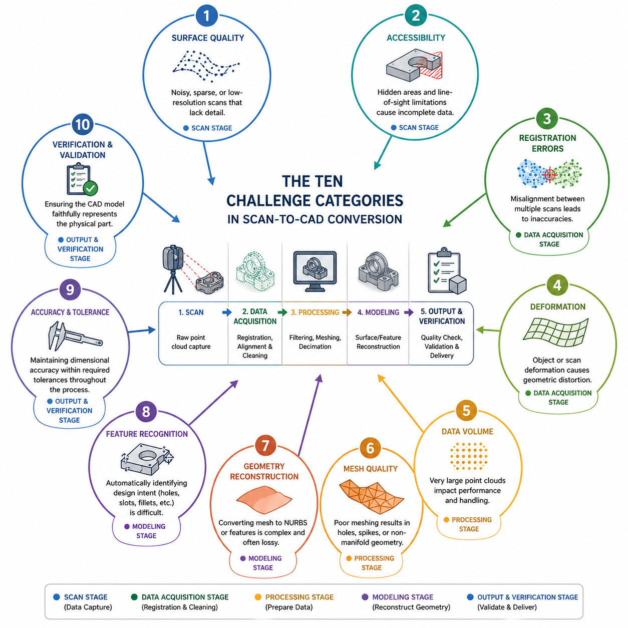
The engineer who has never encountered a scan-to-CAD conversion problem has not done enough scan-to-CAD conversion. The workflow looks straightforward in theory: scan the part, process the data, reconstruct the CAD model. In practice, the gap between those three steps contains ten categories of problems that each have their own technical root cause, their own detection method, and their own fix strategy. Understanding them transforms what feels like a frustrating collection of random failures into a systematic set of manageable engineering challenges.
This article exists because the previous article in this series, covering the complete reverse engineering workflow from scan to CAD model, documents what a successful workflow looks like. This article covers what happens when it does not go according to plan, which in practical engineering work is frequently. The challenges described here are not edge cases. They are the routine obstacles that every engineer executing scan-to-CAD conversion at production quality will encounter within their first ten projects.
Each challenge is covered with the specificity that makes it actionable: the underlying cause that explains why the problem occurs, the detection method that identifies it reliably (because many of these challenges are not immediately obvious), the primary fix strategy, and the alternative approaches when the primary fix is not sufficient or not applicable. The article closes with the legal and intellectual property considerations that every engineer doing competitive reverse engineering must understand, a topic that most technical content on this subject ignores entirely.
Challenge Overview: Root Cause, Detection, and Fix Strategy at a Glance
The following table maps all ten major challenge categories to their root cause, detection method, primary fix strategy, and severity classification. Use it as a quick reference when diagnosing a specific problem, and refer to the detailed section for each challenge for the full technical explanation.
| Challenge | Root Cause | Detection Method | Primary Fix Strategy | Severity |
| Reflective and dark surface scan failure | Specular reflection or light absorption prevents pattern capture | Visual scan gaps, noisy point regions | Matte scanning spray, adjust scanner angle/exposure | High |
| Inaccessible geometry and scan shadows | Line-of-sight limitation of optical scanners | Point cloud gaps after registration | Multi-position scanning, CT for enclosed features | High |
| Part deformation during scanning | Gravity sag or clamping stress in flexible parts | Deviation analysis vs known reference | Fixture design, scan orientation planning | Very High |
| Wear and damage vs original geometry | In-service wear, corrosion, impact damage on scanned part | Statistical analysis of local surface deviation | Comparative measurement, engineering judgment on nominal | Very High |
| Symmetry assumption errors | Engineer assumes symmetry not confirmed in scan data | Mirror comparison deviation analysis | Verify symmetry from scan before applying in CAD | High |
| Thread and fine feature reconstruction | Feature detail finer than scanner resolution | Measured feature depth vs expected | CMM hybrid probing, calculated nominal reconstruction | Medium |
| Data volume and processing performance | High-density scans exceed workstation RAM/CPU capacity | Slow processing, software crashes | Downsampling, workstation spec, SSD storage | Medium |
| Multi-material scan artifacts | Different materials reflect light differently within same scan | Boundary noise at material interfaces | Separate scan sessions per material, CT for embedded parts | High |
| CAD reconstruction quality vs mesh fidelity | Parametric reconstruction cannot capture all mesh detail | Deviation analysis of reconstructed CAD vs mesh | Hybrid approach: parametric for prismatic, NURBS for organic | Medium |
| Color and texture loss in geometry-only formats | STEP and IGES carry no color or texture data | Visual comparison, missing appearance data | Supplement with OBJ+MTL, VRML, or 3D PDF with texture | Low to Medium |
The severity ratings reflect the impact on final CAD model quality if the challenge is not addressed: Very High challenges produce CAD models that are dimensionally incorrect and cannot be used for reproduction or manufacturing without causing failures. High challenges produce models with specific inaccurate regions. Medium challenges degrade model quality or workflow efficiency without necessarily invalidating the output.
Challenge 1: Reflective, Dark, and Transparent Surfaces
Surface optical properties are the most frequently encountered obstacle in structured light and laser line scanning, and they cause the most varied and unpredictable data quality problems. Three distinct surface conditions each create different failure modes: highly reflective surfaces, dark or absorptive surfaces, and transparent or translucent surfaces.
Reflective Surfaces: Specular Glare and Data Voids
Polished metals, chrome plating, mirror finishes, and wet surfaces create specular reflection: they reflect the scanner’s projected light pattern back at a specific angle rather than diffusing it across the field of view. When the camera is not positioned at the exact specular angle, it receives no light from that surface area and records no data. When it is near the specular angle, it receives saturated light that overwhelms the camera sensor, producing blown-out pixels with no useful fringe deformation information.
The characteristic signature of specular reflection in a point cloud is a pattern of voids surrounded by noisy data: the center of the reflection zone has no points (the camera received no return), surrounded by a fringe of noisy points (the camera received partially saturated return with corrupted fringe data). Attempting to fill these voids during mesh repair produces geometrically incorrect surfaces because the hole-filling algorithm has no scan data to work from in that region.
The primary fix is matte scanning spray: a temporary aerosol coating of white titanium dioxide or zinc oxide particles that provides a diffuse, lambertian-reflective surface for consistent light return from any camera angle. Applied correctly in 2 to 3 thin coats from 200 to 300mm distance, the coating is 5 to 15 microns thick and dries to a matte white finish that the scanner reads easily. For most mechanical engineering applications, this coating thickness is negligible relative to part tolerances. For precision surface measurements where the coating thickness matters, use the thinnest possible application and account for the coating thickness in your dimensional analysis.
A secondary approach is to adjust the scanner’s exposure settings to reduce sensitivity and capture less of the saturated reflection, or to reposition the scanner to avoid the specular angle for the most problematic surfaces. Most professional scanning systems allow per-scan exposure adjustment, and some support automatic multi-exposure capture (HDR scanning) that takes multiple exposures in the same position and combines the best data from each, effectively handling mixed reflectivity across a complex surface in a single capture.
Dark and Black Surfaces: Light Absorption
Dark surfaces, particularly matte black coatings, anodized aluminum, carbon fiber, and black rubber, absorb 80 to 95 percent of incident light. The scanner’s projected pattern reaches the surface but the reflected intensity is too low for the camera to detect reliable fringe deformation. The result is sparse, noisy point data rather than complete voids, because some light does return but the signal-to-noise ratio is too low for accurate position calculation.
The fix is the same matte scanning spray, which converts the dark surface to a diffuse white reflector. For parts where spray cannot be used (due to temperature sensitivity, chemical incompatibility, or requirement for an absolutely uncoated surface), alternative approaches include increasing the scanner’s projector intensity (if the system supports it), increasing exposure time, or switching to a laser line scanner rather than a structured light system, as laser line scanners are generally less sensitive to surface color than white-light structured light systems.
Transparent and Translucent Surfaces: Subsurface Scattering
Transparent materials (glass, clear acrylic, polycarbonate lenses) transmit the scanner’s light pattern rather than reflecting it, producing no data at all from the surface. Translucent materials (frosted plastic, skin, some composites) allow light to penetrate the surface and scatter within the material before returning, a phenomenon called subsurface scattering. This produces surface data that is systematically displaced from the true surface position by the scattering depth, typically 0.1 to 2 mm depending on material type and thickness.
Scanning spray converts transparent surfaces to opaque reflectors, resolving both problems. For parts where transparency is a functional property that must be preserved (optical components, light pipes, lenses), CT scanning is the only practical alternative for capturing the surface geometry without any surface preparation.
| Surface Preparation Quick Reference Polished steel, chrome, aluminum mirror finish: 2 to 3 coats matte scanning spray. Anodized aluminum, black paint, carbon fiber: 2 to 3 coats matte scanning spray. Clear glass, polycarbonate, acrylic: 2 to 3 coats matte scanning spray (destroys transparency – use CT if optical function must be preserved). Rubber or silicone: Spray carefully – rubber can absorb spray solvent. Test on an inconspicuous area first. Alternative: use blue LED structured light rather than white LED for better rubber surface response. |
Challenge 2: Inaccessible Geometry and Scan Shadows
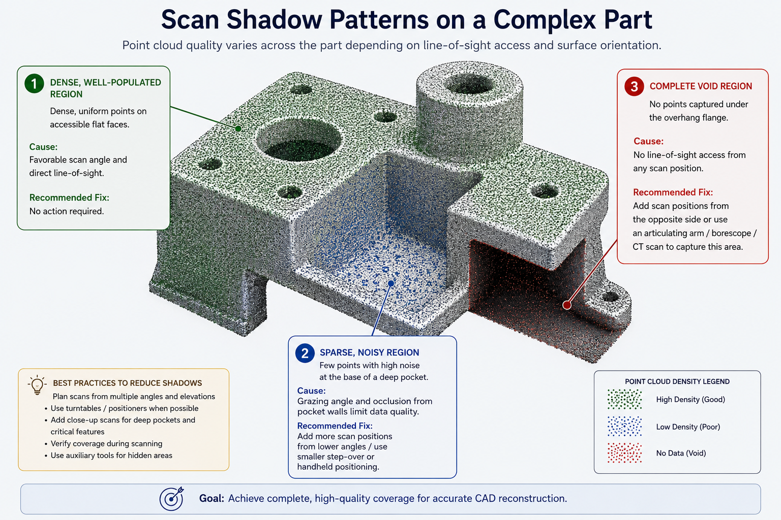
Optical scanners, including structured light, laser line, and photogrammetry systems, share an absolute limitation: they can only capture surfaces they can see. Every feature that is occluded, recessed, or hidden behind another surface during scanning creates a scan shadow: a region of the point cloud with no data because no scan position had line-of-sight access to that surface.
Common examples include the interior of deep pockets, undercut features, the back face of a flange, the interior of a tube or bore, and the region under an overhang. In complex assemblies, adjacent components shadow each other, leaving interface surfaces without scan coverage.
Multi-Position Scanning to Minimize Shadows
The primary strategy for managing scan shadows is systematic multi-position scanning: planning the scan sequence so that every surface receives at least one scan position with acceptable line-of-sight access, even if that position is geometrically difficult to achieve. Before beginning any scan session on a complex part, walk around the part and identify every surface that will be difficult to access optically. Then plan the scanner positions, fixture orientations, and part repositioning steps needed to capture each of those surfaces.
For deep pockets and internal channels, scan from inside the pocket with the scanner tilted to the maximum possible angle. Most structured light systems capture data reliably at angles up to 45 degrees from the surface normal. Beyond this angle, the projected pattern becomes too foreshortened for accurate fringe deformation measurement, and data quality degrades rapidly. Laser line scanners generally have wider acceptance angles and can capture data at 60 to 70 degrees from normal in some configurations.
Industrial CT for Enclosed Internal Geometry
When optical scanning cannot capture required internal geometry regardless of the number of scan positions, industrial CT scanning is the definitive solution. CT sees through the material from all angles simultaneously, capturing internal surfaces, channels, wall thicknesses, and enclosed features that no optical scanner can reach. For hydraulic manifolds, castings with complex internal passages, sealed housings, and any assembly with interior surfaces that define function, CT is not an optional alternative to optical scanning. It is the only technology that captures the complete geometry.
The practical limitation is that CT requires access to a CT system (either in-house or as a service), it is slower than optical scanning, and it has part size constraints. For engineering teams that regularly reverse engineer complex internal geometry, CT scanning as a service from an industrial metrology provider is a practical and cost-effective solution for the cases where optical scanning cannot reach the needed surfaces.
Reconstructing Inaccessible Geometry by Inference
When CT scanning is not available and scan shadows cannot be eliminated through multi-position scanning, the engineer must reconstruct the unseen geometry by inference: using the surrounding scan data to determine what the hidden geometry must be, based on engineering knowledge, visual reference images, or measured cross-sections.
For features that follow predictable manufacturing patterns (a drilled and tapped hole that continues through to a visible back surface, a groove that follows a radius consistent with the cutter diameter visible in the surrounding material, a blind bore whose depth can be estimated from the visible part thickness minus a minimum wall thickness), reasoned reconstruction produces reliable results. For truly arbitrary hidden geometry with no inferential constraints, the CAD model must document the unknown region explicitly in its drawing annotations and inspection requirements.
Challenge 3: Part Deformation During Scanning
Part deformation during scanning is the most damaging challenge in the list because it is invisible in the scan data. The scanner captures the geometry of the part as it actually is during the scan, including any deformation caused by its own weight, by the fixture holding it, or by the thermal environment. The resulting CAD model accurately represents the deformed part, not the part’s true geometry, and the engineer may not discover the problem until a manufactured replacement using the CAD model does not fit correctly.
Gravity Sag in Large or Flexible Parts
Gravity sag is a common deformation mode for large parts, thin flexible sheets, rubber and elastomer components, and any part where the ratio of part mass to stiffness is high enough that measurable deflection occurs under self-weight. A long, thin aluminum extrusion lying horizontally will sag at its center. A rubber seal gasket deforms significantly under its own weight if unsupported. Even a relatively stiff steel bracket can show 50 to 200 microns of sag at its free end when cantilevered, which exceeds the accuracy of a high-quality structured light scan and would produce measurable dimensional error in the resulting CAD model.
The fix is fixture design: supporting the part in a way that replicates its functional configuration, or in a way that eliminates all gravity-induced deflection. For a part that is normally bolted flat to a surface, scan it in that bolted configuration with the mounting surface as the primary datum. For a part whose functional configuration cannot be determined, scan it from multiple orientations and compare the results to identify any gravity-dependent deformation in the data.
Fixture-Induced Stress
Fixtures that clamp or constrain a flexible part to hold it for scanning introduce their own deformation. The clamping force distorts the part geometry in the clamped region and can induce bending or twisting throughout the part. This is particularly problematic for thin-walled plastic parts, sheet metal, and rubber or silicone components. Fixture-induced deformation can be worse than unconstrained gravity sag if the fixture is not designed carefully.
Use the minimum clamping force required to hold the part stable during scanning. For very flexible parts, consider non-contact fixturing: a conformal nest made from foam or sand that supports the part across its full surface without applying point or line loads. For parts where any deformation is unacceptable, use gravity-independent measurement methods: CMM probing with the part in its functional installation configuration, or CT scanning where the part can be scanned while resting naturally without clamping.
Thermal Deformation
Temperature differences between the scan environment and the part’s functional operating temperature cause dimensional changes through thermal expansion. For a 200mm aluminum part (coefficient of thermal expansion approximately 23 microns per millimeter per degree Celsius), a 10 degree Celsius temperature difference between the scan environment and the nominal temperature produces 46 microns of dimensional change, which exceeds the measurement tolerance for precision features.
Ensure the part is at thermal equilibrium with the scan environment before scanning begins. For a part that has been transported from a cold or hot environment, allow 30 to 60 minutes of equilibration time before scanning. For precision work, record the ambient temperature during scanning and apply a thermal expansion correction to the scan data if the scanning temperature differs from the reference temperature (typically 20 degrees Celsius for engineering dimensional measurement per ISO 1 standard).
| Deformation Risk Assessment Low risk: Rigid metal parts under 300mm, wall thickness over 5mm, scanned in ambient conditions. Medium risk: Parts over 500mm, thin-walled structures under 3mm, machined from stock (residual stress). High risk: Rubber/elastomer parts, flexible plastics, large sheet metal, assembled multi-material parts, parts transported from extreme temperatures. For High risk parts: design a dedicated scanning fixture, verify deformation by comparing scans in two different orientations, and consult a metrology engineer before committing the scan data to a CAD reconstruction. |
Challenge 4: Distinguishing Wear and Damage from Original Geometry
This is the most engineering-intensive challenge in the entire scan-to-CAD conversion process because it cannot be resolved by any software tool or measurement technique alone. It requires engineering judgment informed by multiple lines of evidence, and getting it wrong produces a CAD model that faithfully reproduces a damaged part rather than the original design.
The specific problem: the scanned part has been in service and has accumulated geometric changes from in-service wear, impact damage, corrosion, plastic deformation, or fatigue-related distortion. The scan accurately captures the current state of the part, but the reverse engineering goal is typically to reproduce the original design geometry, not the worn state. The scan data alone cannot tell you what is original design geometry and what is accumulated damage.
Types of Geometric Change from Service Life
Abrasive wear produces gradual, smooth reduction in material at contact surfaces. It is typically most severe at sliding interfaces, sealing surfaces, and bearing surfaces. In a scan, worn surfaces appear as slight concavities or reduced thicknesses relative to the expected nominal geometry. Wear patterns are often asymmetric (one side wears faster than the other due to loading direction) and have a smooth, gradual boundary with unworn regions.
Impact damage produces local depressions, cracks, or material loss at specific locations from point loading events. These are typically more localized than wear and have sharper boundaries between damaged and undamaged regions. Impact damage can produce significant local deformations: a 20mm dent in a steel plate from a dropped tool can represent 2 to 5mm of surface displacement.
Corrosion produces surface texture changes and material loss at chemically active surfaces. Early-stage corrosion produces a roughening of the surface texture that increases scan noise without significant dimensional change. Advanced corrosion produces measurable material loss and surface pitting that significantly corrupts the scan data in affected regions.
Plastic deformation from overloading produces permanent geometric change throughout the affected region. Unlike wear (which only removes material from contact surfaces) or impact damage (which is localized), plastic deformation can alter the geometry of large regions of the part in ways that are difficult to identify from the scan alone without reference to the original design dimensions.
Strategies for Identifying Wear and Damage
Use multiple evidence sources in combination to identify which geometric deviations are wear and which are original design features:
- Compare to surviving unworn regions: Most worn parts have some surfaces that were not in contact with anything during service and remain at or near the original geometry. Comparing the worn surfaces to these reference regions establishes what the original dimensions likely were.
- Statistical analysis of the point cloud: Wear and damage produce localized outlier deviations from the general surface geometry. Fitting a geometric primitive to the entire surface and examining the residual deviation distribution identifies regions where the deviation is anomalously large, indicating either damage or an intentional geometric feature. Large, localized positive deviations suggest material buildup or deformation. Large, localized negative deviations suggest wear or removal.
- Multiple part comparison: If more than one example of the same part is available, scanning multiple examples and comparing them isolates genuine design geometry (consistent across all parts) from wear and damage (variable between parts depending on service history).
- Physical reference standards: Assembly drawings, inspection sheets, or supplier part numbers from the original program may establish nominal dimensions against which the scan can be compared, identifying the magnitude and location of all deviations from nominal.
- Manufacturing process inference: An engineer familiar with the manufacturing process for the part type can identify which surfaces would have been machined to a precise nominal and which would have been cast or formed with greater variation. Machined surfaces in an unworn state should have scan residuals close to the scanner’s measurement uncertainty. Larger residuals on machined surfaces indicate either wear or damage.
Challenge 5: The Symmetry Assumption Trap
The symmetry assumption trap is a specific error pattern that is extremely common among engineers who are new to scan-to-CAD conversion and surprisingly persistent among experienced ones. It occurs when an engineer, modeling a part that appears symmetric from visual inspection, applies symmetry in the CAD reconstruction without verifying from the scan data whether the part is actually symmetric within measurement precision. The result is a CAD model that is more symmetric than the physical part, which can cause fit errors in asymmetric assembly interfaces and incorrect mass properties.
Most manufactured parts that are nominally symmetric are not perfectly symmetric in their as-built state. Casting, forging, and injection molding processes all introduce manufacturing variation that is rarely perfectly symmetric. In-service loading can induce asymmetric wear or deformation. And some parts that appear symmetric actually have subtle intentional asymmetry that serves a functional purpose, such as a poka-yoke feature that prevents incorrect installation.
Detecting Asymmetry in Scan Data
The detection method is a mirror comparison analysis: reflect the scan data about the presumed plane of symmetry and compute the deviation between the original data and its mirror image. If the part is truly symmetric within the measurement uncertainty of the scanner, the deviation between original and mirror should be uniformly distributed at or below the scanner’s noise level. If specific regions show systematic deviation above the noise level, those regions are genuinely asymmetric.
Most professional scan processing software (Geomagic, PolyWorks, ZEISS Inspect) includes symmetry analysis tools that perform this comparison automatically and display the results as a color map. This analysis should be performed before any symmetry is applied in the CAD reconstruction, and its results should be documented in the project record.
The Right Response to Detected Asymmetry
When the symmetry analysis reveals asymmetry, the engineer must determine whether it represents manufacturing variation that should be idealized away or intentional design asymmetry that must be preserved. Manufacturing variation is typically random in distribution and magnitude, with no consistent directionality. Intentional design asymmetry is typically consistent across multiple examples of the same part and associated with a functional interface or assembly constraint.
For manufacturing variation: apply symmetry in the CAD model and document the decision with the measured asymmetry magnitude. For intentional asymmetry: model the asymmetric geometry explicitly and investigate whether the asymmetry is a poka-yoke feature, a balancing provision, or a functionally significant geometric difference that affects part performance or assembly.
Challenge 6: Thread and Fine Feature Reconstruction
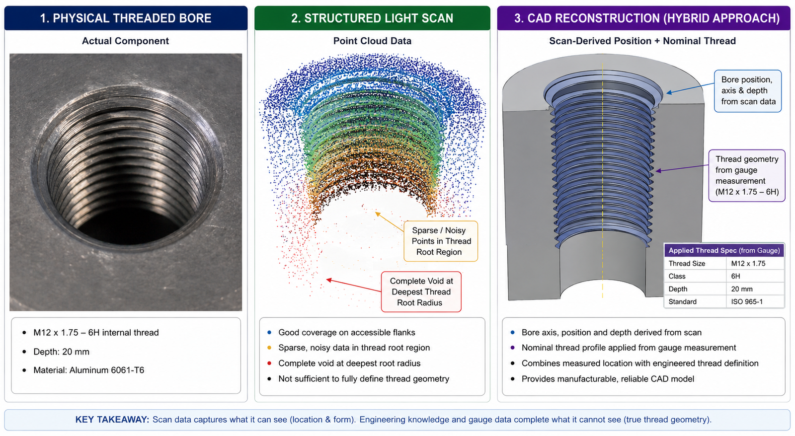
Thread reconstruction from scan data is a universally acknowledged limitation of optical scanning, and it is one area where the standard workflow must be supplemented by a different measurement approach. No current optical 3D scanner reliably captures thread geometry with enough accuracy for thread profile reconstruction. Thread pitches for common metric threads range from 0.35 mm for M2 to 3 mm for M36. The helix angle, flank angle, root radius, and crest geometry of a standard thread are all at a scale that is either below the resolution of most industrial scanners or creates such extreme surface angle variation that the scan data is too noisy to extract meaningful thread geometry.
Why Threads Cannot Be Scanned Reliably
The fundamental problem is geometry, not scanner quality. Thread flanks on a metric thread have a 60-degree included angle, meaning the thread faces are inclined at 30 degrees from the axis. At the root of the thread, the scanner must capture a surface that is deeply recessed between two flanks, at an angle that may exceed the scanner’s angular acceptance. Even when data is captured in the thread region, the thread root and crest radii are typically below the spatial resolution of most structured light systems (typically 0.1 to 0.3 mm point spacing for medium parts). The resulting point cloud in the threaded region is too sparse and noisy to extract reliable thread profile data.
The Hybrid Measurement Approach
The correct approach for threaded features is hybrid measurement: scan the part optically to capture all non-threaded geometry, and measure all threaded features separately using a method appropriate for thread metrology: optical comparator, thread gauge, thread micrometer, or CMM probing with a thread-pitch measuring strategy.
The optical scan provides the position of the threaded bore’s axis (captured from the cylindrical bore surface surrounding the thread), the bore diameter (from the cylinder fit to the major diameter region), and the depth of blind holes. CMM measurement or gauge measurement provides the thread specification: pitch, thread form (metric, UNC, UNF, ACME, etc.), tolerance class, and depth of engagement. The CAD reconstruction combines both sources: the scan-derived position and the gauge-derived thread specification.
Fine Features Below Scanner Resolution
Beyond threads, any geometric feature whose characteristic dimension is smaller than the scanner’s point spacing is potentially affected by resolution-limited reconstruction. Knurling, fine surface textures, small radii (under 0.2 mm), sharp edges (the scanner captures a blend radius that does not exist in the physical part), and fine engraved markings are all below the resolution of most industrial scanners.
For sharp edges and small radii: document the expected nominal value (based on manufacturing process knowledge or reference drawings) and use this nominal value in the CAD model rather than trying to extract it from the scan. A milled part has sharp internal corner radii equal to the end mill radius used. A cast part has minimum radii defined by the mold tool design. These values are more reliably determined from manufacturing process knowledge than from scan data.
Challenge 7: Data Volume and Processing Performance
Modern structured light scanners produce point clouds of 5 to 50 million points per scan position, and complex parts requiring 20 to 40 scan positions produce raw datasets of 100 million to 2 billion points. Processing, registering, and reconstructing CAD geometry from datasets at this scale places substantial demands on workstation hardware, and underpowered workstations are one of the most common practical bottlenecks in scan-to-CAD workflows, causing software crashes, multi-hour processing times for operations that should take minutes, and workflow interruptions that disrupt the engineer’s focus.
The Computational Bottleneck Explained
Point cloud processing operations, particularly ICP registration (which iteratively compares millions of point pairs), mesh generation (which builds topological relationships across hundreds of millions of points), and NURBS surface fitting (which involves large matrix operations), are computationally intensive in specific ways that determine which workstation specifications are most impactful.
RAM is the primary constraint for large dataset operations: a 500-million-point dataset requires 6 to 10 GB of RAM just to hold the point coordinates in memory before any processing begins, and processing operations create temporary copies and work arrays that multiply the memory requirement by 3 to 5 times. Geomagic Design X recommends a minimum of 32 GB RAM for complex scan projects. 64 GB is strongly preferred for large industrial parts. 128 GB is appropriate for very large assemblies or complex organic forms with dense scan data.
CPU performance matters for single-threaded operations like ICP refinement and geometry healing, which benefit from high per-core clock speeds. GPU acceleration is increasingly used by modern scan processing software for mesh generation and surface fitting. Fast NVMe SSD storage is essential because scan datasets routinely exceed the size that fits in RAM and must be streamed from disk during processing. A mechanical hard drive accessing 100 GB of scan data during processing creates wait times that can multiply the total workflow time by 5 to 10 times compared to NVMe storage at the same dataset size.
Practical Strategies for Managing Data Volume
- Uniform downsampling before any processing: Reduce the point cloud to the minimum density that preserves all relevant geometric detail (typically 0.05 to 0.2mm point spacing for industrial parts). This reduction alone cuts processing time by 80 to 95 percent for most operations.
- Region-of-interest processing: Process the scan in sections rather than all at once. Work on each sub-region at the resolution it requires, combining the final processed regions at a later stage.
- 64-bit operating system and application: Verify that the scan processing software is running in 64-bit mode (not 32-bit compatibility mode), which allows access to more than 4 GB of RAM per process.
- Temporary file location: Configure the scan software’s scratch/temporary file directory to point to the fastest available storage (NVMe SSD, not a network drive or mechanical HDD).
- Background process management: Close all non-essential applications during intensive scan processing operations to maximize available RAM and CPU bandwidth for the scan software.
Minimum Workstation Specification for Scan-to-CAD Work |
Challenge 8: Multi-Material Scan Artifacts
Parts made from multiple materials with different optical properties create a specific and often overlooked scan challenge: the scanner is calibrated and optimized for one set of optical conditions, but the part presents multiple different conditions simultaneously. At the boundary between materials with different reflectivity or color, the scanner produces noisy or incorrect data in a zone that extends 1 to 5 millimeters on either side of the material interface.
A metal housing with a rubber gasket face is a classic example. The metal face may require normal exposure settings for the structured light projector. The rubber gasket may require higher exposure and a different angle because it is darker and absorbs more light. At the gasket-to-metal interface, the scan data transitions between these two conditions and produces a noisy boundary zone. The CAD reconstructed from this data shows an inaccurate representation of the interface geometry, which may be the most functionally critical surface in the whole part.
Material Boundary Management Strategies
Strategy 1: Separate scan sessions per material region. Scan the metal faces first with the optimal settings for metal, and the rubber faces in a separate session with adjusted settings. The two sessions are registered together in the same coordinate system using the common coded targets that remain in place throughout both sessions. This approach produces optimal data quality for each material region but requires careful planning to ensure that every surface region belongs clearly to one session or the other, and that enough overlap exists at the boundaries for registration.
Strategy 2: HDR multi-exposure scanning. Some advanced structured light systems support High Dynamic Range scanning, where multiple exposures are taken at each scan position and merged to produce a single point cloud that combines the best data from each exposure level. This effectively handles mixed reflectivity within a single scan session and is the most convenient solution when the equipment supports it.
Strategy 3: Industrial CT for embedded and multi-material assemblies. When the multi-material interface is critical for dimensional accuracy and optical scanning consistently produces poor results at that interface, CT scanning provides accurate geometry for both materials simultaneously, independent of their optical properties. The CT image segments each material based on its X-ray attenuation, which varies by density and atomic composition, providing clean boundaries between material regions even when their optical properties are similar.
Overmolded Parts: A Specific Multi-Material Challenge
Overmolded components, where a soft material is molded over a rigid substrate, present a particular challenge because the soft overmold material deforms differently from the rigid substrate during scanning. If the part is handled or fixtured, the soft overmold deforms at the handling points. If it is scanned without support, gravity causes the overmold to sag. And at the interface between the rigid substrate and the soft overmold, the scan data captures the outer surface of the overmold but provides no information about the substrate geometry beneath it. For overmolded parts where the substrate geometry is functionally critical, CT scanning is the only method that captures both surfaces reliably
Challenge 9: Balancing CAD Model Quality Against Mesh Fidelity
There is an inherent tension in scan-to-CAD conversion between two competing quality goals: geometric fidelity to the scan data and CAD model quality and usability. The mesh produced from the scan data captures every surface irregularity in the physical part: manufacturing variation, surface roughness, minor damage, and scan noise are all present in the mesh as genuine geometric features. A CAD model that precisely reproduces every detail of the mesh is geometrically accurate to the scan but may be extremely difficult to use for design modification, drawing generation, or FEA because of its complexity and lack of parametric structure.
The engineer must make deliberate decisions about how much mesh detail to preserve in the CAD model and how much to idealize. These decisions should be documented so that anyone reviewing the CAD model can understand what level of idealization was applied and what the underlying scan data showed.
The Four Levels of Mesh Detail in CAD Reconstruction
Level 1: Exact mesh representation – The mesh itself is the CAD output. No parametric reconstruction is performed. The mesh is cleaned, repaired, and exported as STL, OBJ, or similar format. Appropriate when the output is for 3D printing, visualization, or simulation where mesh input is accepted and parametric CAD is not required.
Level 2: NURBS surface fit to mesh – NURBS surfaces are fitted to the mesh regions, capturing the general shape including manufacturing variation. The resulting surfaces are smooth but not perfectly prismatic. Appropriate for organic forms and consumer product surfaces where the general manufactured shape is what needs to be captured.
Level 3: Fitted primitives with as-built dimensions – Geometric primitives (planes, cylinders, spheres) are fitted to the mesh and the as-built dimensions are extracted. The CAD model uses these as-built values directly as driving dimensions. Appropriate for exact reproduction where every dimensional deviation from nominal is intentional and must be preserved.
Level 4: Idealized parametric reconstruction – Geometric primitives are fitted to the mesh, nominal dimensions are inferred by rounding to standard values, and the CAD model is built as a fully parametric part with clean feature tree, named parameters, and nominal dimensions. Appropriate for design intent recovery and downstream modification.
The choice between these levels should be made explicitly at the beginning of the project based on the engineering intent defined in the previous article. Defaulting to Level 4 for all projects adds unnecessary modeling time. Defaulting to Level 1 produces output that is often unusable for engineering purposes. Matching the level to the application makes the project efficient and the output fit for purpose.
Challenge 10: Legal and Intellectual Property Considerations
This challenge is categorically different from the nine technical challenges above. It is not a data quality problem or a workflow efficiency problem. It is a legal risk that applies specifically to competitive reverse engineering: the process of scanning and recreating a product manufactured by another organization for the purpose of understanding, competing with, or reproducing that product.
Most scan-to-CAD content for engineers treats this topic as outside scope. That is a significant disservice, because engineers executing competitive reverse engineering programs without understanding the applicable legal framework are exposing their organizations to significant liability. The legal landscape is complex, jurisdiction-dependent, and evolving, and this article is not a substitute for qualified legal advice. But the framework below provides the starting orientation that every engineer doing competitive reverse engineering needs.
What Is and Is Not Protected by Intellectual Property Law
Patents protect functional inventions for a limited term (typically 20 years from filing). A patented mechanism, assembly method, or process cannot be reproduced without a license regardless of how the reproduction is achieved, including by scanning the patented product. Before conducting reverse engineering of a competitor’s product, check whether the functional aspects of interest are patented in the jurisdictions where the reproduction will be manufactured and sold.
Trade dress protects the distinctive visual appearance of a product or its packaging. If the exterior appearance of a product has been registered as trade dress, creating a CAD model that reproduces that appearance and using it to manufacture a competing product may infringe the trade dress even if the functional geometry is not patented.
Copyrights do not typically protect functional three-dimensional objects (as opposed to artistic or sculptural works), but software embedded in a product, digital design files obtained directly from a manufacturer, and decorative or artistic surface features may be copyright-protected.
Trade secrets protect confidential information that has economic value from its secrecy. If information about a product was obtained through a confidential relationship (such as a supplier agreement that included non-disclosure obligations), using that information in a reverse engineering program may breach the confidentiality agreement regardless of whether the information itself is patented.
The Legitimate Uses of Competitive Reverse Engineering
In most jurisdictions, reverse engineering a legally purchased product for interoperability, compatibility, or research purposes is a legally protected activity, provided the product was purchased lawfully and no contractual restriction on analysis was agreed to at purchase. Manufacturing and selling a competing product that reproduces patented functionality is not protected. Manufacturing and selling a competing product that provides the same function through a non-infringing design (informed by understanding the competitor’s approach through reverse engineering) is generally protected.
The practical implication for engineering teams is: document the purpose of the reverse engineering program clearly at its outset. Engineering understanding of a competitor’s design approach for the purpose of designing a non-infringing alternative is legally very different from engineering a direct copy. If the purpose is not clearly documented, a court may draw unfavorable inferences about intent from the existence of scan data and CAD models of a competitor’s product.
| Legal Caution This section provides only a general orientation to intellectual property considerations in reverse engineering. It does not constitute legal advice. Before committing to any competitive reverse engineering program that will result in a commercial product, consult qualified intellectual property counsel in the relevant jurisdictions. The legal framework varies significantly between countries (particularly between the US, EU, and Asian jurisdictions), between industries, and based on the specific facts of each situation. |
Frequently Asked Questions
Q: Why do I get holes and voids in my 3D scan data?
Holes and voids in 3D scan data have three main causes: line-of-sight limitations (the scanner cannot see surfaces hidden behind other geometry), surface optical properties (reflective surfaces create specular glare voids, dark surfaces create sparse data, transparent surfaces produce no data), and scanner standoff angle violations (data captured at too shallow an angle to the surface produces noise or voids). The fix depends on the cause: add scan positions to reach hidden surfaces, apply matte scanning spray for optical surface issues, or use industrial CT scanning for enclosed internal features that optical scanners cannot reach.
Q: How do I scan reflective metal parts without getting glare artifacts?
Apply a matte anti-glare scanning spray (titanium dioxide or zinc oxide aerosol) to the reflective surface in 2 to 3 thin coats from 200 to 300mm distance. The 5 to 15 micron coating provides a diffuse, lambertian-reflective surface that the structured light scanner can capture accurately from any angle. The coating is temporary and can be washed off after scanning with water or a mild solvent. For highly polished precision surfaces where coating thickness matters, apply the thinnest possible coat and account for the coating thickness (typically 5 to 10 microns) in your dimensional analysis. Alternative approaches include HDR multi-exposure scanning or adjusting the scanner angle to avoid the specular reflection zone.
Q: Can I accurately reconstruct thread dimensions from a 3D scan?
No, optical 3D scanning cannot reliably capture thread geometry at the accuracy required for thread specification reconstruction. Thread pitches for common fasteners range from 0.35mm to 3mm, and the thread root radius and flank geometry are at a scale below the resolution of most industrial scanners. The correct approach is hybrid measurement: scan the part optically to capture the bore position and major diameter, then measure the thread specification separately using a thread gauge, optical comparator, or CMM probing. Combine both data sources in the CAD reconstruction: scan-derived position and gauge-derived thread specification.
Q: How do I tell whether a dimensional deviation in my scan is wear or original design geometry?
Compare the deviation against multiple evidence sources: surviving unworn surfaces on the same part (which should remain near the original design geometry), statistical analysis of the point cloud to identify systematic vs random deviations (wear is typically smooth and directional, design features are consistent and bounded), comparison across multiple examples of the same part if available (wear varies with service history, design features are consistent), and manufacturing process inference (machined surfaces should have scan residuals near the scanner noise level if unworn). When in doubt, document the uncertainty explicitly and flag the affected dimensions for verification before any manufacturing commitment.
Q: What workstation specifications do I need for scan-to-CAD work?
For medium-complexity industrial parts producing 50 to 500 million points: 64 GB RAM (minimum, 128 GB preferred), Intel i9 or AMD Threadripper CPU with 16+ cores, NVIDIA RTX 4080 or better GPU with at least 16 GB VRAM, and NVMe SSD storage for both the operating system and project data. RAM is the primary bottleneck: scan processing creates multiple temporary copies of large datasets simultaneously. NVMe SSD storage is the second most impactful specification because large datasets must be streamed from disk during processing. A mechanical hard drive accessing large scan data can multiply total processing time by 5 to 10 compared to NVMe storage.
Q: Is reverse engineering a competitor’s product legal?
It depends on the jurisdiction and the specific purpose. In most jurisdictions, reverse engineering a legally purchased product for purposes of interoperability, research, or designing a non-infringing alternative is a legally protected activity. However, reproducing patented functionality, infringing registered trade dress, or using information obtained under a confidentiality obligation can create significant legal liability regardless of how the reverse engineering was conducted. The specific legal framework varies between countries and industries. Before commencing any competitive reverse engineering program intended to result in a commercial product, obtain qualified legal advice from intellectual property counsel in the relevant jurisdictions. Document the purpose of the program clearly at its outset.
Q: Why does my CAD model not match the scan data in the final deviation analysis?
Large deviation analysis discrepancies have several common causes: incorrect primitive fitting (the plane or cylinder fit did not capture the true geometry of that region), design intent rounding to nominal that moved a dimension outside the measurement uncertainty range, part deformation during scanning that was not detected and corrected, wear or damage on the scanned part that was inadvertently reproduced in the CAD model, or a registration error in the point cloud that introduced a systematic misalignment. The deviation analysis color map identifies exactly where the CAD model deviates from the scan. Return to the reconstruction for each high-deviation region and re-examine the fitting or modeling decision that produced the deviation.
Conclusion:
The ten challenges covered in this article account for the overwhelming majority of the problems that engineers encounter in scan-to-CAD conversion workflows. None of them are random or unpredictable. Each has a specific root cause that explains why it occurs, a specific detection method that identifies it before it corrupts the final output, and a specific fix strategy that resolves it when it is detected.
The pattern across all ten challenges is consistent: problems that are detected early in the workflow are solved cheaply. Problems that reach the CAD reconstruction stage, or worse, the deviation analysis stage, are solved expensively. Surface preparation before scanning is ten minutes. Discovering missing scan data after the scanner has been returned to its case and the part has been cleaned is a rescan request. Detecting asymmetry before applying symmetry in CAD is a five-minute analysis. Discovering the asymmetry error after completing the parametric reconstruction is an hours-long rework.
Build the pre-scan checklist, the intermediate quality checks, and the final deviation analysis into every scan-to-CAD project as non-negotiable workflow steps. The engineers who execute scan-to-CAD conversion at the highest reliability are not the ones who never encounter these challenges. They are the ones who detect and address each challenge at the earliest possible workflow stage, before it becomes a project-level problem.
Build your complete scan-to-CAD knowledge with our guide to the full reverse engineering workflow, CAD data translation problems, parametric modeling best practices, and multi-body modeling techniques.
Leave a Reply